Chapter 3 Functional Programming

3.1 Introduction

3.1.1 Function definitions

As mentioned in the functional programming overview functional programming is one of the numerous ways to write code. In functional programming, you write functions that do the computations and then as the user, you call these functions to work for you.

You should be familiar with function definitions in R. For example, suppose you want to compute the square root of a number and want to do so using Newton’s algorithm:

sqrt_newton <- function(a, init, eps = 0.01){
    while(abs(init**2 - a) > eps){
        init <- 1/2 *(init + a/init)
    }
    return(init)
}

You can then use this function to get the square root of a number:

sqrt_newton(16, 2)

## [1] 4.00122

We are using a while loop inside the body. The body of a function are the instructions that define the function. You can get the body of a function with body(some_func)] of the function. In pure functional programming languages, like Haskell, you don’t have loops. How can you program without loops, you may ask? In functional programming, loops are replaced by recursion. Let’s rewrite our little example above with recursion:

sqrt_newton_recur <- function(a, init, eps = 0.01){
    if(abs(init**2 - a) < eps){
        result <- init
    } else {
        init <- 1/2 * (init + a/init)
        result <- sqrt_newton_recur(a, init, eps)
    }
    return(result)
}

sqrt_newton_recur(16, 2)

## [1] 4.00122

R is not a pure functional programming language though, so we can still use loops (be it while or for loops) in the bodies of our functions. Actually, for R specifically, it is better, performance-wise, to use loops instead of recursion, because R is not tail-call optimized. I won’t got into the details of what tail-call optimization is but just remember that if performance is important a loop will be faster. However, sometimes, it is easier to write a function using recursion. I personally tend to avoid loops if performance is not important, because I find that code that avoids loops is easier to read and debug. However, knowing that you have can use loops is reassuring. In the coming sections I will show you some built-in function that make it possible to avoid writing loops and that don’t rely on recursion, so performance won’t be penalized.

3.1.2 Properties of functions

Mathematical functions have a nice property: we always get the same output for a given input. This is called referential transparency and we should aim to write our R functions in such a way.

For example, the following function:

increment <- function(x){
    return(x + 1)
}

Is a referential transparent function. We always get the same result for any x that we give to this function.

This:

increment(10)

## [1] 11

will always produce 11.

However, this one:

increment_opaque <- function(x){
    return(x + spam)
}

is not a referential transparent function, because its value depends on the global variable spam.

spam <- 1

increment_opaque(10)

## [1] 11

will only produce 11 if spam = 1. But what if spam = 19?

spam <- 19

increment_opaque(10)

## [1] 29

To make increment_opaque() a referential transparent function, it is enough to make spam an argument:

increment_not_opaque <- function(x, spam){
    return(x + spam)
}

Now even if there is a global variable called spam, this will not influence our function:

spam <- 19

increment_not_opaque(10, 34)

## [1] 44

This is because the variable spam defined in the body of the function is a local variable. It could have been called anything else, really. Avoiding opaque functions makes our life easier.

Another property that adepts of functional programming value is that functions should have no, or very limited, side-effects. This means that functions should not change the state of your program.

For example this function (which is not a referential transparent function):

count_iter <- 0

sqrt_newton_side_effect <- function(a, init, eps = 0.01){
    while(abs(init**2 - a) > eps){
        init <- 1/2 *(init + a/init)
        count_iter <<- count_iter + 1 # The "<<-" symbol means that we assign the
    }                                 # RHS value in a variable in the global environment
    return(init)
}

If you look in the environment pane, you will see that count_iter equals 0. Now call this function with the following arguments:

sqrt_newton_side_effect(16000, 2)

## [1] 126.4911

print(count_iter)

## [1] 9

If you check the value of count_iter now, you will see that it increased! This is a side effect, because the function changed something outside its scope. It changed a value in the global environment. In general, it is good practice to avoid side-effects. For example, we could make the above function not have any side effects like this:

sqrt_newton_count <- function(a, init, count_iter = 0, eps = 0.01){
    while(abs(init**2 - a) > eps){
        init <- 1/2 *(init + a/init)
        count_iter <- count_iter + 1
    }
    return(c(init, count_iter))
}

Now, this function returns a list with two elements, the result, and the number of iterations it took to get the result:

sqrt_newton_count(16000, 2)

## [1] 126.4911   9.0000

Writing to disk is also considered a side effect, because the function changes something (a file) outside its scope. But this cannot be avoided (and it’s actually a good thing to have, functions that can write to disk) so just remember: try to avoid having functions changing variables in the global environment unless you have a very good reason of doing so.

Finally, another property of mathematical functions, is that they do one single thing. Functional programming purists also program their functions to do one single task. This has benefits, but can complicate things. The function we wrote previously does two things: it computes the square root of a number and also returns the number of iterations it took to compute the result. However, this is not a bad thing; the function is doing two tasks, but these tasks are related to each other and it makes sense to have them together. My piece of advice: avoid having functions that do too many unrelated things. This makes debugging harder.

In conclusion: you should strive for referential transparency, try to avoid side effects unless you have a good reason to have them and try to keep your functions short and do as little tasks as possible. This makes testing and debugging easier, as you will see.

3.2 Mapping and Reducing: the base way

No introduction to functional programming would be complete without some discussion about the functions Map() (and the associated *apply() family of functions) and Reduce(). Map() allows you to map your function to every element of a list of arguments and is easy to understand, while Reduce() (sometimes called fold() in other programming languages) reduces a list of values to a single value by successively applying a function. It’s a bit harder to understand, but with some examples it will become clear soon enough. In this section we will focus on how to do things using base functions. In the next section we will take a look at the purrr package which extends R’s functional programming capabilities tremendously.

3.2.1 Mapping with `Map()` and the `*apply()` family of functions

Now that we have our nice function that computes square roots using Newton’s algorithm, we would like to compute the square root of every element in the following list:

numbers <- c(16, 25, 36, 49, 64, 81)

sqrt_newton(numbers, init = rep(1, 6), eps = rep(0.001, 6))

## Warning in while (abs(init^2 - a) > eps) {: the condition has length > 1
## and only the first element will be used

## Warning in while (abs(init^2 - a) > eps) {: the condition has length > 1
## and only the first element will be used

## Warning in while (abs(init^2 - a) > eps) {: the condition has length > 1
## and only the first element will be used

## Warning in while (abs(init^2 - a) > eps) {: the condition has length > 1
## and only the first element will be used

## Warning in while (abs(init^2 - a) > eps) {: the condition has length > 1
## and only the first element will be used

## Warning in while (abs(init^2 - a) > eps) {: the condition has length > 1
## and only the first element will be used

## [1] 4.000001 5.000023 6.000253 7.001406 8.005148 9.014272

We get a whole bunch of nasty warning messages, but we do get the expected result. But you should not leave it like this. Who knows what may happen some time down the road, when you try to compose this function with another? Maybe you’ll get an error and you won’t understand why! Let’s rewrite the function properly.

We get these warnings because the condition (init^2 - a) > eps does not make sense for vectors. Here, R tells the user that it only uses the first element and then does the computation anyways. I would prefer if R would stop the execution and print an error message. This would force the user to have to rewrite the function to explicitly take vectors into account. And there is a very simple way of doing it, by using the function Map():

Map(sqrt_newton, numbers, init = 1)

## [[1]]
## [1] 4.000001
## 
## [[2]]
## [1] 5.000023
## 
## [[3]]
## [1] 6.000253
## 
## [[4]]
## [1] 7
## 
## [[5]]
## [1] 8.000002
## 
## [[6]]
## [1] 9.000011

Map() applies a function to every element of a list and returns a list.

We could then write a wrapper around Map():

sqrt_newton_vec <- function(numbers, init, eps = 0.01){
    return(Map(sqrt_newton, numbers, init, eps))
}

sqrt_newton_vec(numbers, 1)

## [[1]]
## [1] 4.000001
## 
## [[2]]
## [1] 5.000023
## 
## [[3]]
## [1] 6.000253
## 
## [[4]]
## [1] 7
## 
## [[5]]
## [1] 8.000002
## 
## [[6]]
## [1] 9.000011

As you can see, we can give a function as an argument to another function. This makes Map() a higher-order function. Higher-order functions are functions that take other functions as arguments and return either another function, or a value. This is another important concept in functional programming and encourages modularity. It makes your code easily reusable!

R has other higher-order functions that work like Map(), such as apply(), lapply(), mapply(), sapply(), vapply() and tapply(). Depending on what you want to do, you will have to use one or the other. apply() and ‘tapply()’ are different from the other *apply() functions, because they work on arrays. You can apply a function on the rows or columns of an array, for example if you want a row-wise sum:

a <- cbind(c(1, 2, 3), c(4, 5, 6), c(7, 8, 9))
apply(a, 1, sum)

## [1] 12 15 18

We could use lapply() instead of Map():

lapply(numbers, sqrt_newton, init = 1)

## [[1]]
## [1] 4.000001
## 
## [[2]]
## [1] 5.000023
## 
## [[3]]
## [1] 6.000253
## 
## [[4]]
## [1] 7
## 
## [[5]]
## [1] 8.000002
## 
## [[6]]
## [1] 9.000011

or sapply():

sapply(numbers, sqrt_newton, init = 1)

## [1] 4.000001 5.000023 6.000253 7.000000 8.000002 9.000011

We could rewrite sqrt_newton_vec() with sapply() which would return a better looking result (a list of numbers instead of a list of lists):

sqrt_newton_vec <- function(numbers, init, eps = 0.01){
    return(sapply(numbers, sqrt_newton, init, eps))
}

sqrt_newton_vec(numbers, 1)

## [1] 4.000001 5.000023 6.000253 7.000000 8.000002 9.000011

mapply() is different from these two:

inits <- c(100, 20, 3212, 487, 5, 9888)
mapply(sqrt_newton, numbers, init = inits)

## [1] 4.000284 5.000001 6.000003 7.000006 8.000129 9.000006

What happens here is that sqrt_newton() gets called with following arguments:

sqrt_newton(numbers[1], inits[1])

## [1] 4.000284

sqrt_newton(numbers[2], inits[2])

## [1] 5.000001

sqrt_newton(numbers[3], inits[3])

## [1] 6.000003

sqrt_newton(numbers[4], inits[4])

## [1] 7.000006

sqrt_newton(numbers[5], inits[5])

## [1] 8.000129

sqrt_newton(numbers[6], inits[6])

## [1] 9.000006

From the Map()’s documentation, we learn that:

`Map()` is wrapper to `mapply()` which does not attempt to simplify the result...

All this behaviour can be replicated using loops, but once you get the gist of these functions, you can write code that is shorter and easier to read and unlike in the case of recursion, without any loss in performance (but without any gains either).

3.2.2 `Reduce()`

Reduce() is another very useful higher-order function, especially if you want to avoid loops to make your code easier to read. In some programming languages, Reduce() is called fold().

I think that the following example illustrates the power of Reduce() well:

Reduce(`+`, numbers, init = 0)

## [1] 271

Can you guess what happens? Reduce() takes a function as an argument, here the function +¹ and then does the following computation:

0 + numbers[1] + numbers[2] + numbers[3]...

It applies the user supplied function successively but has to start with something, so we give it the argument init also. This argument is actually optional, but I show it here because in some cases it might be useful to start the computations at another value than 0. This function generalizes functions that only take two arguments. If you were to write a function that returns the minimum between two numbers:

my_min <- function(a, b){
    if(a < b){
        return(a)
    } else {
        return(b)
    }
}

You could use Reduce() to get the minimum of a list of numbers:

print(numbers)

## [1] 16 25 36 49 64 81

Reduce(my_min, numbers)

## [1] 16

Here we don’t supply an init because there is no need for it. Of course R’s built-in min() function works on a list of values. But Reduce() is a very powerful function that can make our life much easier and most importantly avoid writing clumsy loops.

3.3 Mapping and Reducing: the `purrr` way

Hadley Wickham developed a package called purrr which contains a lot of very useful functions. I will show some of them here, but in the next chapter, we are going to study purrr in greater depth. Also, take the time to read purrr’s documentation, and of course you can read more about purrr in Wickham and Grolemund (2016).

3.3.1 The `map*()` family of functions

In the previous section we saw how to map a function to each element of a list. Each version of an *apply() function has a different purpose, but it is not very easy to remember which one returns a list, which other one returns an atomic vector and so on. If you’re working on data frames you can use apply() to sum (for example) over columns or rows, because you can specify which MARGIN you want to sum over. But you do not get a data frame back. In the purrr package, each of the functions that do mapping have a similar name. The first part of these functions’ names all start with map_ and the second part tells you what this function is going to output. For example, if you want doubles out, you would use map_dbl(). If you are working on data frames want a data frame back, you would use map_df(). These are much more intuitive and easier to remember and we’re going to learn how to use them in the chapter about The Tidyverse. For now, let’s just focus on the basic functions, map() and reduce() (and some variants of reduce()). To map a function to every element of a list, simply use map():

library("purrr")
map(numbers, sqrt_newton, init = 1)

## [[1]]
## [1] 4.000001
## 
## [[2]]
## [1] 5.000023
## 
## [[3]]
## [1] 6.000253
## 
## [[4]]
## [1] 7
## 
## [[5]]
## [1] 8.000002
## 
## [[6]]
## [1] 9.000011

Compared to Map(), the function and the list are given in the reverse order, but the result is the same, of course.

3.3.2 Reducing with `purrr`

In the purrr package, you can find two more functions for folding: reduce() and reduce_right(). The difference between reduce() and reduce_right() is pretty obvious: reduce_right() starts from the right!

a <- seq(1, 10)

reduce(a, `-`)

## [1] -53

reduce_right(a, `-`)

## [1] -35

For operations that are not commutative, this makes a difference. Other interesting folding functions are accumulate() and accumulate_right():

a <- seq(1, 10)

accumulate(a, `-`)

##  [1]   1  -1  -4  -8 -13 -19 -26 -34 -43 -53

accumulate_right(a, `-`)

##  [1] -35 -34 -32 -29 -25 -20 -14  -7   1  10

These two functions keep the intermediary results.

3.4 Basic anonymous functions

One last very useful concept are anonymous functions. Suppose that you want to apply one of your own functions to a list of datasets. For instance, you want to have a histogram of a variable that is called the same accross a list of datasets. Maybe your datasets are yearly surveys and each year the survey was conducted is another .csv file. For illustration purposes, let us use the mtcars dataset with some minor changes:

data(mtcars)

mtcars2000 <- mtcars
mtcars2001 <- mtcars
mtcars2001$cyl <- mtcars2001$cyl+3
datasets <- list("mtcars2000" = mtcars2000,
"mtcars2001" = mtcars2001)

In the next chapters we will learn how to load a lot of datasets at once and store them in a list. So it is important to know how to work with datasets that are stored on lists. Now suppose you want to use purrr::map() to plot a histogram of variable cyl for each dataset that is contained in your list.

map(datasets, hist, cyl)

Error in hist.default(.x[[i]], ...) : 'x' must be numeric

Maybe try this:

map(datasets, hist(cyl))

Error in hist(cyl) : object 'cyl' not found

So how can we solve this issue? One way is to use an anonymous function. Anonymous functions are functions that get declared on the fly and do not have names. These are especially useful inside higher order functions such as purrr::map():

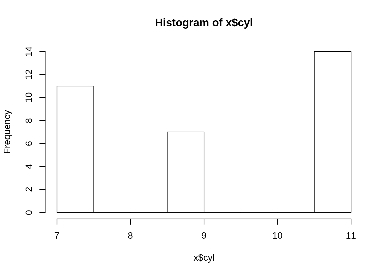
map(datasets, (function(x) hist(x$cyl)))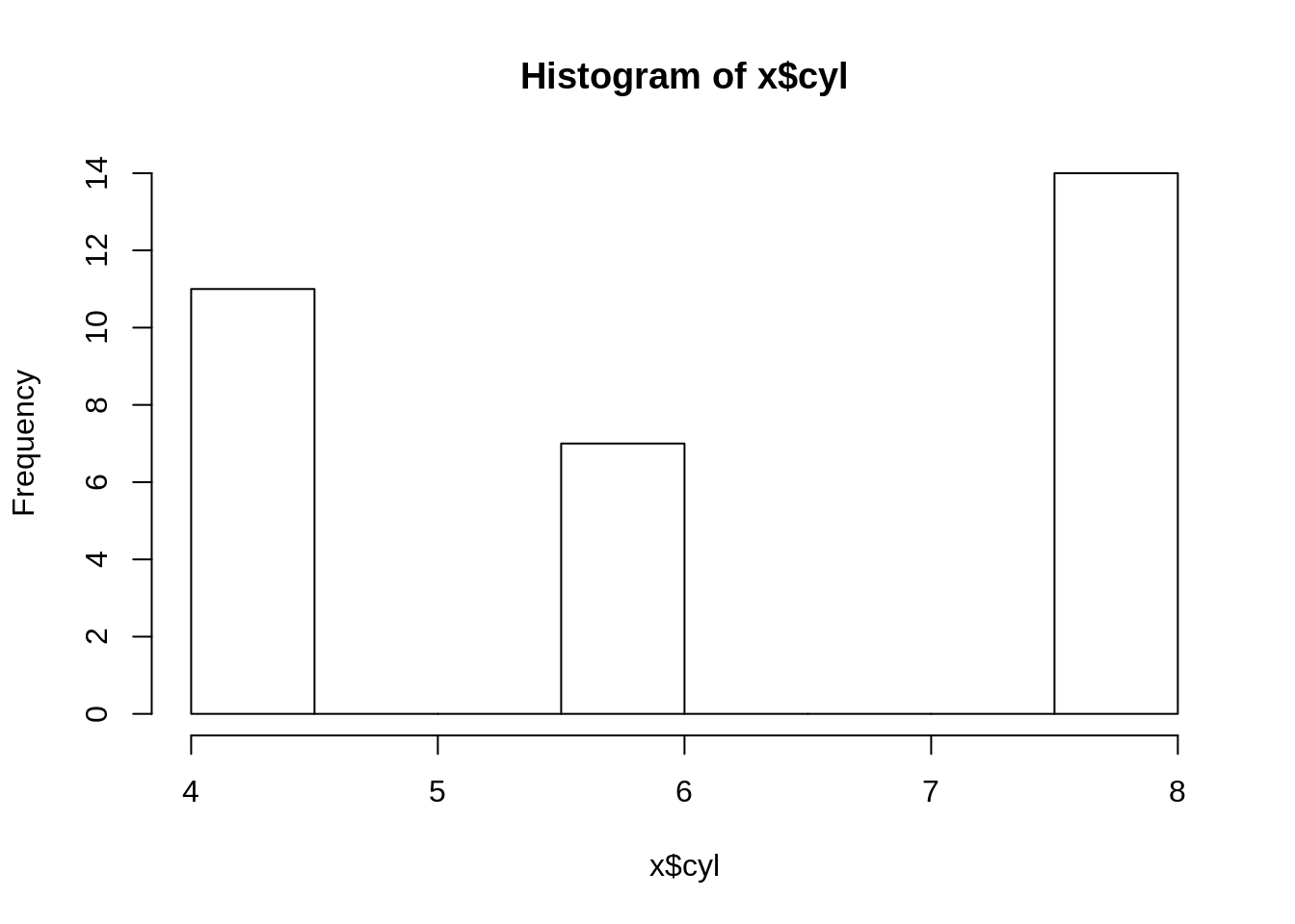

## $mtcars2000
## $breaks
## [1] 4.0 4.5 5.0 5.5 6.0 6.5 7.0 7.5 8.0
## 
## $counts
## [1] 11  0  0  7  0  0  0 14
## 
## $density
## [1] 0.6875 0.0000 0.0000 0.4375 0.0000 0.0000 0.0000 0.8750
## 
## $mids
## [1] 4.25 4.75 5.25 5.75 6.25 6.75 7.25 7.75
## 
## $xname
## [1] "x$cyl"
## 
## $equidist
## [1] TRUE
## 
## attr(,"class")
## [1] "histogram"
## 
## $mtcars2001
## $breaks
## [1]  7.0  7.5  8.0  8.5  9.0  9.5 10.0 10.5 11.0
## 
## $counts
## [1] 11  0  0  7  0  0  0 14
## 
## $density
## [1] 0.6875 0.0000 0.0000 0.4375 0.0000 0.0000 0.0000 0.8750
## 
## $mids
## [1]  7.25  7.75  8.25  8.75  9.25  9.75 10.25 10.75
## 
## $xname
## [1] "x$cyl"
## 
## $equidist
## [1] TRUE
## 
## attr(,"class")
## [1] "histogram"

Here the function is enclosed between () and is not named. The function has a single argument x, which is supposed to be a dataset. We then plot a histogram of the variable cyl from this dataset. Then this function is mapped to every dataset contained in the list datasets that we created above.

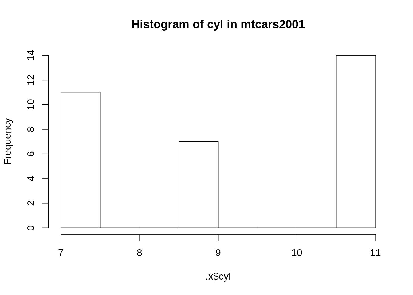
We can also write anonymous functions that are more complex:

map2(
.x = datasets, .y = names(datasets),
(function(.x, .y) hist(.x$cyl, main=paste("Histogram of cyl in", .y)))
)

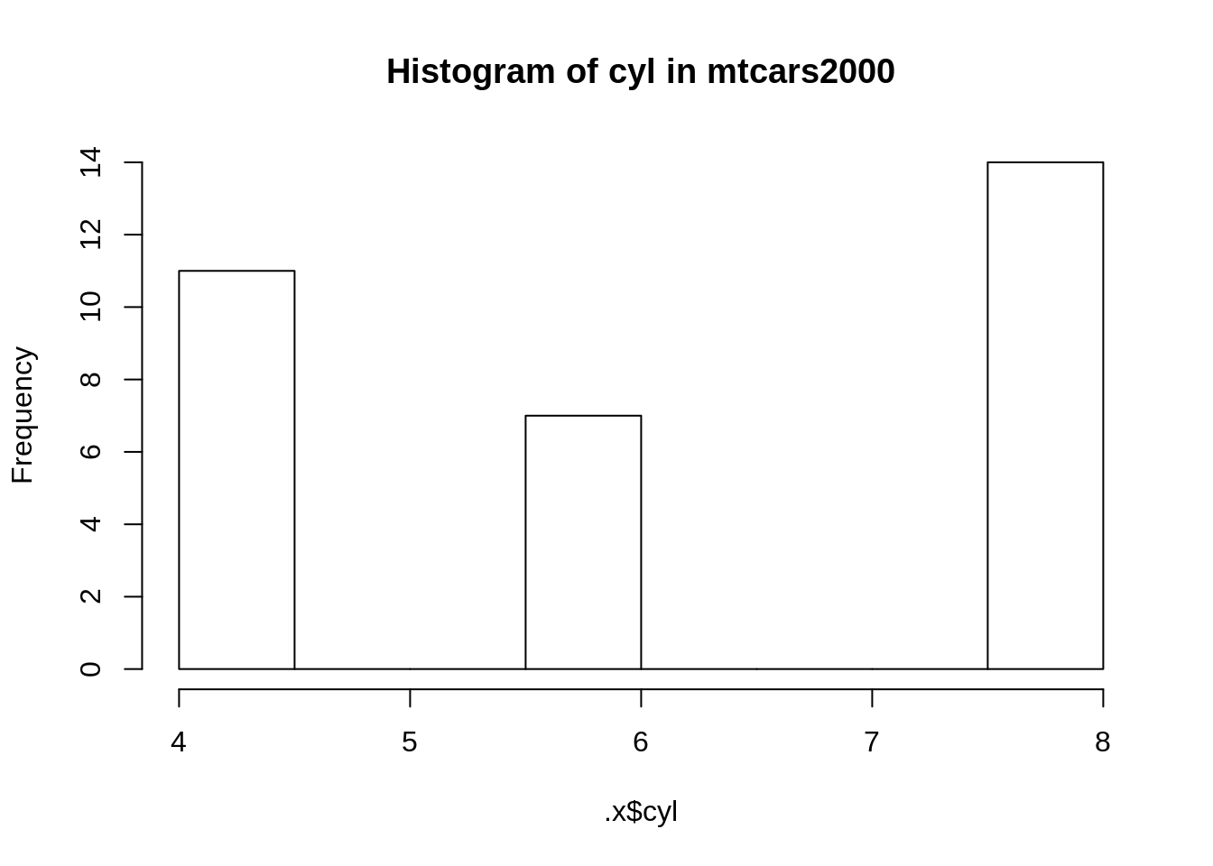
## $mtcars2000
## $breaks
## [1] 4.0 4.5 5.0 5.5 6.0 6.5 7.0 7.5 8.0
## 
## $counts
## [1] 11  0  0  7  0  0  0 14
## 
## $density
## [1] 0.6875 0.0000 0.0000 0.4375 0.0000 0.0000 0.0000 0.8750
## 
## $mids
## [1] 4.25 4.75 5.25 5.75 6.25 6.75 7.25 7.75
## 
## $xname
## [1] ".x$cyl"
## 
## $equidist
## [1] TRUE
## 
## attr(,"class")
## [1] "histogram"
## 
## $mtcars2001
## $breaks
## [1]  7.0  7.5  8.0  8.5  9.0  9.5 10.0 10.5 11.0
## 
## $counts
## [1] 11  0  0  7  0  0  0 14
## 
## $density
## [1] 0.6875 0.0000 0.0000 0.4375 0.0000 0.0000 0.0000 0.8750
## 
## $mids
## [1]  7.25  7.75  8.25  8.75  9.25  9.75 10.25 10.75
## 
## $xname
## [1] ".x$cyl"
## 
## $equidist
## [1] TRUE
## 
## attr(,"class")
## [1] "histogram"

Of course you could have defined the anonymous function as a regular function before using map(). But sometimes it is faster to simply use an anonymous function as long as it does not hurt clarity.

This is the end of the introduction to functional programming. Entire books have been written on the subject, such as the upcoming book by Khan (2017) or Lipovaca (2011). If you’re curious about functional programming, you should read these books. For our purposes though, knowing how to write functions, and trying to make them referentially transparent as well as knowing about mapping and reducing is enough to get us going.

3.5 Wrap-up

Make your functions referentially transparent.
Avoid side effects (if possible).
Make your functions do one thing (if possible).
A function that takes another function as an argument is called an higher-order function. You can write your own higher-order functions and this is a way of having short and easily testable functions. Making these functions then work together is trivial and is what makes functional programming very powerful.

3.6 Exercises

For the following exercises, you will have to use any of the functions that we saw in this chapter. Reduce(), Map() or any function from the *apply() family of functions. Do not use loops! If you don’t know how to solve these exercises wait for the next section, where we’ll learn how to write unit tests. Writing unit tests before the functions they’re supposed to test is called test-driven development and can help you write your functions.

Create a function that returns the factorial of a number using Reduce(). Remember: no recursion nor loops allowed!

my_fact(5)

[1] 120

Suppose you have a list of data set names. Create a function that removes “.csv” from each of these names. Start by creating a function that does so using stri_split() from the package stringi (you can also use strsplit() from base R). Below is an illustration of how it’s supposed to work:

dataset_names <- c("dataset1.csv", "dataset2.csv", "dataset3.csv")

remove_csv(dataset_names)

[1] "dataset1" "dataset2" dataset3"

Create a function that takes a number a, and then returns either the sum of the numbers from 1 to this number that are divisible by another number b or the product of the numbers from 1 to this number that are divisible by b. Your function should be a higher-order function with the following arguments: a the number, divisible_func the function that checks whether a number is divisible by some number b and reduce_op the function that either sums or multiplies the numbers from 1 to a that are divisible by b.

reduce_some_numbers(a = 10, divisible_func = divisible, b = 2, reduce_op = `*`)

[1] 3840

References

Wickham, Hadley, and Garrett Grolemund. 2016. R for Data Science. 1st ed. O’Reilly. http://r4ds.had.co.nz/.

Khan, Aslam. 2017. Grokking Functional Programming. 1st ed. Manning Publications. https://www.manning.com/books/grokking-functional-programming.

Lipovaca, Miran. 2011. Learn You a Haskell for Great Good!: A Beginner’s Guide. no starch press. http://learnyouahaskell.com/.

This is simply the + operator you’re used to. Try this out: `+`(1, 5) and you’ll see + is a function like any other. You just have to write backticks around the plus symbol to make it work.↩