Chapter 4 The tidyverse
The tidyverse is the name given to a certain number of packages, most of all (if not all?) developed by, or co-developed by, Hadley Wickham. There’s a website that introduces them all: The tidyverse. In this chapter, we are going to learn about some functions of some of these packages. We already know a little bit about purrr; let’s discover what these other packages have to offer!
However, before reading everything that follows, I’d suggest you watch Hadley Wickham’s talk Expressing yourself with R. R is a computer language, and as with any language we really are writing things that are supposed to be read and understood by others, not just the computer. Even if you’re working alone, you owe it to your future self to write clean, easy to understand code. Using the tidyverse and adopting the principles presented in the talk will put you in the right mindset for everything that follows!
First of all, let’s install the tidyverse packages. You can install them one by one, or you can install the tidyverse meta-package:
install.packages("tidyverse")I suggest you do just that, as we’re going to skim over all the packages. To start an analysis, we first have to import data into R.
4.1 Smoking is bad for you, but pipes are your friend
The title of this section might sound weird at first, but by the end of it, you’ll get this (terrible) pun.
You probably know the following painting by René Magritte, La trahison des images:
knitr::include_graphics("assets/pas_une_pipe.png")
It turns out there’s an R package from the tidyverse that is called magrittr. What does this package do? It brings pipes to R. Pipes are a concept from the Unix operating system; if you’re using a GNU+Linux distribution or macOS, you’re basically using a modern unix. (That’s an oversimplification, but I’m an economist by training, and outrageously oversimplifying things is what we do, deal with it.)
The idea of pipes is to take the output of a command, and feed it as the input of another command. The magrittr package brings pipes to R, by using the weird looking %>%. Try the following:
library(magrittr)16 %>% sqrt## [1] 4Super weird right? But you probably understand what happened; 16 got fed as the first argument of the function sqrt(). You can chain multiple functions:
16 %>% sqrt %>% `+`(18)## [1] 22The output of 16 (16) got fed to sqrt(), and the output of sqrt(16) (4) got fed to +(18) (22). Without %>% you’d write the line just above like this:
sqrt(16) + 18## [1] 22It might not be very clear right now why this is useful, but the %>% is probably one of the best things that R has, because when using packages from the tidyverse, you will naturally want to chain a lot of functions together. Without the %>% it would become messy very fast.
%>% is not the only pipe operator in magrittr. There’s %T%, %<>% and %$%. All have their uses, but are basically shortcuts to some common tasks with %>% plus another function. Which means that you can live without them, and because of this, I will only discuss them briefly once we’ll have learned about the other tidyverse packages.
4.2 Getting data into R with readr, readxl, haven and what are tibbles
You probably already know how to import data in R, but maybe you are not familiar with these packages. Using them is pretty straightforward, and I will only discuss haven a little bit more than readr or readxl. readr allows you to import *.csv files as well as other files in plain text. The functions included in readr are fairly straightforward, but there is an aspect that I really like about them: if they fail to read your data you can get a report of what went wrong with the problems() function. I suggest you read the Data import chapter of R for Data Science, to get to know readr better. But for our purposes, knowing the basic read_csv() function is enough.
readxl is very similar to readr but focuses on importing Excel sheets into R. Read more about it on the tidyverse website.
haven imports data from STATA, SAS and SPSS. I’m going into a bit more detail here, by showing an example with a STATA file. STATA files are usually labelled, and I’d like to show how to work with these labels using R. We’re going to work with the mtcars dataset. I used STATA 14 to label the variables; so the dataset looks like one you could have to work with one day.
mtcars_stata <- haven::read_dta("assets/mtcars.dta")
head(mtcars_stata)
## # A tibble: 6 x 12
## car mpg cyl disp hp drat wt qsec vs am
## <chr> <dbl> <dbl> <dbl> <dbl> <dbl> <dbl> <dbl> <dbl> <dbl>
## 1 Mazda RX4 21.0 6 160 110 3.90 2.620 16.46 0 1
## 2 Mazda RX4 Wag 21.0 6 160 110 3.90 2.875 17.02 0 1
## 3 Datsun 710 22.8 4 108 93 3.85 2.320 18.61 1 1
## 4 Hornet 4 Drive 21.4 6 258 110 3.08 3.215 19.44 1 0
## 5 Hornet Sportabout 18.7 8 360 175 3.15 3.440 17.02 0 0
## 6 Valiant 18.1 6 225 105 2.76 3.460 20.22 1 0
## # ... with 2 more variables: gear <dbl>, carb <dbl>You don’t see it here, but the columns are labelled. Try the following:
str(mtcars_stata$car)## atomic [1:32] Mazda RX4 Mazda RX4 Wag Datsun 710 Hornet 4 Drive ...
## - attr(*, "label")= chr "Make and model of the car"
## - attr(*, "format.stata")= chr "%19s"As you can see, the car column has the label attribute, which equals “Make and model of the car”. The other columns are also labelled:
str(mtcars_stata$cyl)## atomic [1:32] 6 6 4 6 8 6 8 4 4 6 ...
## - attr(*, "label")= chr "Number of cylinders"
## - attr(*, "format.stata")= chr "%8.0g"str(mtcars_stata$am)## atomic [1:32] 1 1 1 0 0 0 0 0 0 0 ...
## - attr(*, "label")= chr "Transmission (0 = automatic, 1 = manual)"
## - attr(*, "format.stata")= chr "%8.0g"Another way to get the label is to use the attr() function:
attr(mtcars_stata$cyl, "label")## [1] "Number of cylinders"Let’s use what we learned until now to get the labels of all the columns:
show_labels <- function(dataset){
  map(dataset, function(col)(attr(col, "label")))
}

show_labels(mtcars_stata)
## $car
## [1] "Make and model of the car"
##
## $mpg
## [1] "Miles/(US) gallon"
##
## $cyl
## [1] "Number of cylinders"
##
## $disp
## [1] "Displacement (cu.in.)"
##
## $hp
## [1] "Gross horsepower"
##
## $drat
## [1] "Rear axle ratio"
##
## $wt
## [1] "Weight (1000 lbs)"
##
## $qsec
## [1] "1/4 mile time"
##
## $vs
## [1] "V/S"
##
## $am
## [1] "Transmission (0 = automatic, 1 = manual)"
##
## $gear
## [1] "Number of forward gears"
##
## $carb
## [1] "Number of carburetors"Could we label any dataset and then export it to a .dta file and have the labels in STATA? Let’s find out with the cars dataset:
data(cars)

attr(cars$speed, "label") <- "Speed (mph)"
attr(cars$dist, "label") <- "Stopping distance (feet)"

haven::write_dta(cars, "assets/cars.dta")
Below you see that cars.dta file opened in STATA:
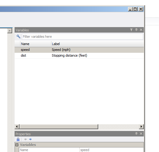
When you use any of the discussed packages to import data, the resulting object is a tibble. tibbles are modern day ‘data.frame’s. The first thing you might have noticed is when you print a tibble vs a ’data.frame’:
data(mtcars)

print(mtcars)
## mpg cyl disp hp drat wt qsec vs am gear carb
## Mazda RX4 21.0 6 160.0 110 3.90 2.620 16.46 0 1 4 4
## Mazda RX4 Wag 21.0 6 160.0 110 3.90 2.875 17.02 0 1 4 4
## Datsun 710 22.8 4 108.0 93 3.85 2.320 18.61 1 1 4 1
## Hornet 4 Drive 21.4 6 258.0 110 3.08 3.215 19.44 1 0 3 1
## Hornet Sportabout 18.7 8 360.0 175 3.15 3.440 17.02 0 0 3 2
## Valiant 18.1 6 225.0 105 2.76 3.460 20.22 1 0 3 1
## Duster 360 14.3 8 360.0 245 3.21 3.570 15.84 0 0 3 4
## Merc 240D 24.4 4 146.7 62 3.69 3.190 20.00 1 0 4 2
## Merc 230 22.8 4 140.8 95 3.92 3.150 22.90 1 0 4 2
## Merc 280 19.2 6 167.6 123 3.92 3.440 18.30 1 0 4 4
## Merc 280C 17.8 6 167.6 123 3.92 3.440 18.90 1 0 4 4
## Merc 450SE 16.4 8 275.8 180 3.07 4.070 17.40 0 0 3 3
## Merc 450SL 17.3 8 275.8 180 3.07 3.730 17.60 0 0 3 3
## Merc 450SLC 15.2 8 275.8 180 3.07 3.780 18.00 0 0 3 3
## Cadillac Fleetwood 10.4 8 472.0 205 2.93 5.250 17.98 0 0 3 4
## Lincoln Continental 10.4 8 460.0 215 3.00 5.424 17.82 0 0 3 4
## Chrysler Imperial 14.7 8 440.0 230 3.23 5.345 17.42 0 0 3 4
## Fiat 128 32.4 4 78.7 66 4.08 2.200 19.47 1 1 4 1
## Honda Civic 30.4 4 75.7 52 4.93 1.615 18.52 1 1 4 2
## Toyota Corolla 33.9 4 71.1 65 4.22 1.835 19.90 1 1 4 1
## Toyota Corona 21.5 4 120.1 97 3.70 2.465 20.01 1 0 3 1
## Dodge Challenger 15.5 8 318.0 150 2.76 3.520 16.87 0 0 3 2
## AMC Javelin 15.2 8 304.0 150 3.15 3.435 17.30 0 0 3 2
## Camaro Z28 13.3 8 350.0 245 3.73 3.840 15.41 0 0 3 4
## Pontiac Firebird 19.2 8 400.0 175 3.08 3.845 17.05 0 0 3 2
## Fiat X1-9 27.3 4 79.0 66 4.08 1.935 18.90 1 1 4 1
## Porsche 914-2 26.0 4 120.3 91 4.43 2.140 16.70 0 1 5 2
## Lotus Europa 30.4 4 95.1 113 3.77 1.513 16.90 1 1 5 2
## Ford Pantera L 15.8 8 351.0 264 4.22 3.170 14.50 0 1 5 4
## Ferrari Dino 19.7 6 145.0 175 3.62 2.770 15.50 0 1 5 6
## Maserati Bora 15.0 8 301.0 335 3.54 3.570 14.60 0 1 5 8
## Volvo 142E 21.4 4 121.0 109 4.11 2.780 18.60 1 1 4 2print(mtcars_stata)## # A tibble: 32 x 12
## car mpg cyl disp hp drat wt qsec vs am
## <chr> <dbl> <dbl> <dbl> <dbl> <dbl> <dbl> <dbl> <dbl> <dbl>
## 1 Mazda RX4 21.0 6 160.0 110 3.90 2.620 16.46 0 1
## 2 Mazda RX4 Wag 21.0 6 160.0 110 3.90 2.875 17.02 0 1
## 3 Datsun 710 22.8 4 108.0 93 3.85 2.320 18.61 1 1
## 4 Hornet 4 Drive 21.4 6 258.0 110 3.08 3.215 19.44 1 0
## 5 Hornet Sportabout 18.7 8 360.0 175 3.15 3.440 17.02 0 0
## 6 Valiant 18.1 6 225.0 105 2.76 3.460 20.22 1 0
## 7 Duster 360 14.3 8 360.0 245 3.21 3.570 15.84 0 0
## 8 Merc 240D 24.4 4 146.7 62 3.69 3.190 20.00 1 0
## 9 Merc 230 22.8 4 140.8 95 3.92 3.150 22.90 1 0
## 10 Merc 280 19.2 6 167.6 123 3.92 3.440 18.30 1 0
## # ... with 22 more rows, and 2 more variables: gear <dbl>, carb <dbl>Only the first 10 lines of the tibble get printed, but the number of remaining lines and the names of the columns that didn’t find are shown as well as the types of the columns.
You can easily create a tibble from vectors:
library(tibble)

set.seed(123)
example <- tibble(a = seq(1,5), b = rnorm(5), c = rpois(5, 3))

print(example)
## # A tibble: 5 x 3
## a b c
## <int> <dbl> <int>
## 1 1 -0.56047565 6
## 2 2 -0.23017749 3
## 3 3 1.55870831 4
## 4 4 0.07050839 3
## 5 5 0.12928774 1Even better than print(), there’s glimpse():
glimpse(mtcars_stata)## Observations: 32
## Variables: 12
## $ car <chr> "Mazda RX4", "Mazda RX4 Wag", "Datsun 710", "Hornet 4 Dri...
## $ mpg <dbl> 21.0, 21.0, 22.8, 21.4, 18.7, 18.1, 14.3, 24.4, 22.8, 19....
## $ cyl <dbl> 6, 6, 4, 6, 8, 6, 8, 4, 4, 6, 6, 8, 8, 8, 8, 8, 8, 4, 4, ...
## $ disp <dbl> 160.0, 160.0, 108.0, 258.0, 360.0, 225.0, 360.0, 146.7, 1...
## $ hp <dbl> 110, 110, 93, 110, 175, 105, 245, 62, 95, 123, 123, 180, ...
## $ drat <dbl> 3.90, 3.90, 3.85, 3.08, 3.15, 2.76, 3.21, 3.69, 3.92, 3.9...
## $ wt <dbl> 2.620, 2.875, 2.320, 3.215, 3.440, 3.460, 3.570, 3.190, 3...
## $ qsec <dbl> 16.46, 17.02, 18.61, 19.44, 17.02, 20.22, 15.84, 20.00, 2...
## $ vs <dbl> 0, 0, 1, 1, 0, 1, 0, 1, 1, 1, 1, 0, 0, 0, 0, 0, 0, 1, 1, ...
## $ am <dbl> 1, 1, 1, 0, 0, 0, 0, 0, 0, 0, 0, 0, 0, 0, 0, 0, 0, 1, 1, ...
## $ gear <dbl> 4, 4, 4, 3, 3, 3, 3, 4, 4, 4, 4, 3, 3, 3, 3, 3, 3, 4, 4, ...
## $ carb <dbl> 4, 4, 1, 1, 2, 1, 4, 2, 2, 4, 4, 3, 3, 3, 4, 4, 4, 1, 2, ...tibbles are lazy, which means that something like this is valid:
set.seed(123)
example <- tibble(a = seq(1,5), b = rnorm(5), c = 10 * b)

glimpse(example)
## Observations: 5
## Variables: 3
## $ a <int> 1, 2, 3, 4, 5
## $ b <dbl> -0.56047565, -0.23017749, 1.55870831, 0.07050839, 0.12928774
## $ c <dbl> -5.6047565, -2.3017749, 15.5870831, 0.7050839, 1.2928774The tibble package contains some other useful functions, such as tribble(), which allows you to create a tibble row by row:
set.seed(123)

example <- tribble(
  ~a, ~b, ~c,
  1, 2, "spam",
  3, 4, "eggs",
  5, 6, "bacon"
)

glimpse(example)
## Observations: 3
## Variables: 3
## $ a <dbl> 1, 3, 5
## $ b <dbl> 2, 4, 6
## $ c <chr> "spam", "eggs", "bacon"Another thing I find very useful is the following:
mtcars$m## [1] 21.0 21.0 22.8 21.4 18.7 18.1 14.3 24.4 22.8 19.2 17.8 16.4 17.3 15.2
## [15] 10.4 10.4 14.7 32.4 30.4 33.9 21.5 15.5 15.2 13.3 19.2 27.3 26.0 30.4
## [29] 15.8 19.7 15.0 21.4mtcars_stata$m## Warning: Unknown or uninitialised column: 'm'.## NULLmtcars$m shows the mpg column… for some reason. There might be a good reason for this, but I prefer tibbles’ behaviour of notifying the user that this column does not exist.
It is possible to convert a lot of objects into tibbles:
example <- matrix(rnorm(36), nrow = 6)

as_tibble(example)
## # A tibble: 6 x 6
## V1 V2 V3 V4 V5 V6
## <dbl> <dbl> <dbl> <dbl> <dbl> <dbl>
## 1 -0.56047565 0.4609162 0.4007715 0.7013559 -0.6250393 0.4264642
## 2 -0.23017749 -1.2650612 0.1106827 -0.4727914 -1.6866933 -0.2950715
## 3 1.55870831 -0.6868529 -0.5558411 -1.0678237 0.8377870 0.8951257
## 4 0.07050839 -0.4456620 1.7869131 -0.2179749 0.1533731 0.8781335
## 5 0.12928774 1.2240818 0.4978505 -1.0260044 -1.1381369 0.8215811
## 6 1.71506499 0.3598138 -1.9666172 -0.7288912 1.2538149 0.6886403example_df <- as.data.frame(example)
as_tibble(example_df)## # A tibble: 6 x 6
## V1 V2 V3 V4 V5 V6
## <dbl> <dbl> <dbl> <dbl> <dbl> <dbl>
## 1 -0.56047565 0.4609162 0.4007715 0.7013559 -0.6250393 0.4264642
## 2 -0.23017749 -1.2650612 0.1106827 -0.4727914 -1.6866933 -0.2950715
## 3 1.55870831 -0.6868529 -0.5558411 -1.0678237 0.8377870 0.8951257
## 4 0.07050839 -0.4456620 1.7869131 -0.2179749 0.1533731 0.8781335
## 5 0.12928774 1.2240818 0.4978505 -1.0260044 -1.1381369 0.8215811
## 6 1.71506499 0.3598138 -1.9666172 -0.7288912 1.2538149 0.6886403example_list <- list(a = seq(1,5), b = seq(6, 10))
as_tibble(example_list)## # A tibble: 5 x 2
## a b
## <int> <int>
## 1 1 6
## 2 2 7
## 3 3 8
## 4 4 9
## 5 5 10You can also convert named vectors to tibbles with enframe:
recipe <- c("spam" = 1, "eggs" = 3, "bacon" = 10)

enframe(recipe, "ingredients", "quantity")
## # A tibble: 3 x 2
## ingredients quantity
## <chr> <dbl>
## 1 spam 1
## 2 eggs 3
## 3 bacon 10Contrast this to as_tibble() or as as.data.frame():
as.data.frame(recipe)## recipe
## spam 1
## eggs 3
## bacon 10as_tibble(recipe)## # A tibble: 3 x 1
## value
## * <dbl>
## 1 1
## 2 3
## 3 10There are a lot of other functions in the tibble package that you might find useful. I suggest you take a look at all of them and see what you can integrate in your workflow!
4.2.1 The swiss army knife of data import and export: rio
rio is a package that is not part of the tidyverse, but it is so useful that I simply cannot not write about it. rio is a metapackage that downloads and installs a whole lot of packages to import and export data, and uses these packages under the hood to import any kind of dataset.
To import data with rio, import() is all you need:
library(rio)

mtcars = import("rio_datasets/mtcars.csv")head(mtcars)## mpg cyl disp hp drat wt qsec vs am gear carb
## 1 21.0 6 160 110 3.90 2.620 16.46 0 1 4 4
## 2 21.0 6 160 110 3.90 2.875 17.02 0 1 4 4
## 3 22.8 4 108 93 3.85 2.320 18.61 1 1 4 1
## 4 21.4 6 258 110 3.08 3.215 19.44 1 0 3 1
## 5 18.7 8 360 175 3.15 3.440 17.02 0 0 3 2
## 6 18.1 6 225 105 2.76 3.460 20.22 1 0 3 1import() needs the path to the data, and you can specify additional options if needed. Importing a STATA or a SAS file is done just the same:
mtcars_stata = import("rio_datasets/mtcars.dta")
head(mtcars_stata)
## mpg cyl disp hp drat wt qsec vs am gear carb
## 1 21.0 6 160 110 3.90 2.620 16.46 0 1 4 4
## 2 21.0 6 160 110 3.90 2.875 17.02 0 1 4 4
## 3 22.8 4 108 93 3.85 2.320 18.61 1 1 4 1
## 4 21.4 6 258 110 3.08 3.215 19.44 1 0 3 1
## 5 18.7 8 360 175 3.15 3.440 17.02 0 0 3 2
## 6 18.1 6 225 105 2.76 3.460 20.22 1 0 3 1mtcars_sas = import("rio_datasets/mtcars.sas7bdat")
head(mtcars_sas)## mpg cyl disp hp drat wt qsec vs am gear carb
## 1 21.0 6 160 110 3.90 2.620 16.46 0 1 4 4
## 2 21.0 6 160 110 3.90 2.875 17.02 0 1 4 4
## 3 22.8 4 108 93 3.85 2.320 18.61 1 1 4 1
## 4 21.4 6 258 110 3.08 3.215 19.44 1 0 3 1
## 5 18.7 8 360 175 3.15 3.440 17.02 0 0 3 2
## 6 18.1 6 225 105 2.76 3.460 20.22 1 0 3 1It is also possible to import Excel files where each sheet is a single table, but you will need import_list() for that. The file multi.xlsx has two sheets, each with a table in it:
multi = import_list("rio_datasets/multi.xlsx")
str(multi)
## List of 2
## $ :'data.frame': 32 obs. of 11 variables:
## ..$ mpg : num [1:32] 21 21 22.8 21.4 18.7 18.1 14.3 24.4 22.8 19.2 ...
## ..$ cyl : num [1:32] 6 6 4 6 8 6 8 4 4 6 ...
## ..$ disp: num [1:32] 160 160 108 258 360 ...
## ..$ hp : num [1:32] 110 110 93 110 175 105 245 62 95 123 ...
## ..$ drat: num [1:32] 3.9 3.9 3.85 3.08 3.15 2.76 3.21 3.69 3.92 3.92 ...
## ..$ wt : num [1:32] 2.62 2.88 2.32 3.21 3.44 ...
## ..$ qsec: num [1:32] 16.5 17 18.6 19.4 17 ...
## ..$ vs : num [1:32] 0 0 1 1 0 1 0 1 1 1 ...
## ..$ am : num [1:32] 1 1 1 0 0 0 0 0 0 0 ...
## ..$ gear: num [1:32] 4 4 4 3 3 3 3 4 4 4 ...
## ..$ carb: num [1:32] 4 4 1 1 2 1 4 2 2 4 ...
## $ :'data.frame': 150 obs. of 5 variables:
## ..$ Sepal.Length: num [1:150] 5.1 4.9 4.7 4.6 5 5.4 4.6 5 4.4 4.9 ...
## ..$ Sepal.Width : num [1:150] 3.5 3 3.2 3.1 3.6 3.9 3.4 3.4 2.9 3.1 ...
## ..$ Petal.Length: num [1:150] 1.4 1.4 1.3 1.5 1.4 1.7 1.4 1.5 1.4 1.5 ...
## ..$ Petal.Width : num [1:150] 0.2 0.2 0.2 0.2 0.2 0.4 0.3 0.2 0.2 0.1 ...
## ..$ Species : chr [1:150] "setosa" "setosa" "setosa" "setosa" ...As you can see multi is a list of datasets. Told you lists were very flexible! It is also possible to import all the datasets in a single directory at once. For this, you first need a vector of paths:
paths = Sys.glob("rio_datasets/unemployment/*.csv")Sys.glob() allows you to find files using a regular expression. “rio_datasets/unemployment/*.csv" matches all the .csv files inside “rio_datasets/unemployment”.
all_data = import_list(paths)

str(all_data)
## List of 4
## $ :'data.frame': 118 obs. of 8 variables:
## ..$ Commune : chr [1:118] "Grand-Duche de Luxembourg" "Canton Capellen" "Dippach" "Garnich" ...
## ..$ Total employed population : int [1:118] 223407 17802 1703 844 1431 4094 2146 971 1218 3002 ...
## ..$ of which: Wage-earners : int [1:118] 203535 15993 1535 750 1315 3800 1874 858 1029 2664 ...
## ..$ of which: Non-wage-earners: int [1:118] 19872 1809 168 94 116 294 272 113 189 338 ...
## ..$ Unemployed : int [1:118] 19287 1071 114 25 74 261 98 45 66 207 ...
## ..$ Active population : int [1:118] 242694 18873 1817 869 1505 4355 2244 1016 1284 3209 ...
## ..$ Unemployment rate (in %) : num [1:118] 7.95 5.67 6.27 2.88 4.92 ...
## ..$ Year : int [1:118] 2013 2013 2013 2013 2013 2013 2013 2013 2013 2013 ...
## $ :'data.frame': 118 obs. of 8 variables:
## ..$ Commune : chr [1:118] "Grand-Duche de Luxembourg" "Canton Capellen" "Dippach" "Garnich" ...
## ..$ Total employed population : int [1:118] 228423 18166 1767 845 1505 4129 2172 1007 1268 3124 ...
## ..$ of which: Wage-earners : int [1:118] 208238 16366 1606 757 1390 3840 1897 887 1082 2782 ...
## ..$ of which: Non-wage-earners: int [1:118] 20185 1800 161 88 115 289 275 120 186 342 ...
## ..$ Unemployed : int [1:118] 19362 1066 122 19 66 287 91 38 61 202 ...
## ..$ Active population : int [1:118] 247785 19232 1889 864 1571 4416 2263 1045 1329 3326 ...
## ..$ Unemployment rate (in %) : num [1:118] 7.81 5.54 6.46 2.2 4.2 ...
## ..$ Year : int [1:118] 2014 2014 2014 2014 2014 2014 2014 2014 2014 2014 ...
## $ :'data.frame': 118 obs. of 8 variables:
## ..$ Commune : chr [1:118] "Grand-Duche de Luxembourg" "Canton Capellen" "Dippach" "Garnich" ...
## ..$ Total employed population : int [1:118] 233130 18310 1780 870 1470 4130 2170 1050 1300 3140 ...
## ..$ of which: Wage-earners : int [1:118] 212530 16430 1620 780 1350 3820 1910 920 1100 2770 ...
## ..$ of which: Non-wage-earners: int [1:118] 20600 1880 160 90 120 310 260 130 200 370 ...
## ..$ Unemployed : int [1:118] 18806 988 106 29 73 260 80 41 72 169 ...
## ..$ Active population : int [1:118] 251936 19298 1886 899 1543 4390 2250 1091 1372 3309 ...
## ..$ Unemployment rate (in %) : num [1:118] 7.46 5.12 5.62 3.23 4.73 ...
## ..$ Year : int [1:118] 2015 2015 2015 2015 2015 2015 2015 2015 2015 2015 ...
## $ :'data.frame': 118 obs. of 8 variables:
## ..$ Commune : chr [1:118] "Grand-Duche de Luxembourg" "Canton Capellen" "Dippach" "Garnich" ...
## ..$ Total employed population : int [1:118] 236100 18380 1790 870 1470 4160 2160 1030 1330 3150 ...
## ..$ of which: Wage-earners : int [1:118] 215430 16500 1640 780 1350 3840 1900 900 1130 2780 ...
## ..$ of which: Non-wage-earners: int [1:118] 20670 1880 150 90 120 320 260 130 200 370 ...
## ..$ Unemployed : int [1:118] 18185 975 91 27 66 246 76 35 70 206 ...
## ..$ Active population : int [1:118] 254285 19355 1881 897 1536 4406 2236 1065 1400 3356 ...
## ..$ Unemployment rate (in %) : num [1:118] 7.15 5.04 4.84 3.01 4.3 ...
## ..$ Year : int [1:118] 2016 2016 2016 2016 2016 2016 2016 2016 2016 2016 ...In a subsequent chapter we will learn how to actually use these lists of datasets.
If you know that each dataset in each file has the same colmuns, you can also import them directly into a single dataset by binding each dataset together using rbind = TRUE:
bind_data = import_list(paths, rbind = TRUE)
str(bind_data)
## 'data.frame': 472 obs. of 9 variables:
## $ Commune : chr "Grand-Duche de Luxembourg" "Canton Capellen" "Dippach" "Garnich" ...
## $ Total employed population : int 223407 17802 1703 844 1431 4094 2146 971 1218 3002 ...
## $ of which: Wage-earners : int 203535 15993 1535 750 1315 3800 1874 858 1029 2664 ...
## $ of which: Non-wage-earners: int 19872 1809 168 94 116 294 272 113 189 338 ...
## $ Unemployed : int 19287 1071 114 25 74 261 98 45 66 207 ...
## $ Active population : int 242694 18873 1817 869 1505 4355 2244 1016 1284 3209 ...
## $ Unemployment rate (in %) : num 7.95 5.67 6.27 2.88 4.92 ...
## $ Year : int 2013 2013 2013 2013 2013 2013 2013 2013 2013 2013 ...
## $ _file : chr "rio_datasets/unemployment/unemp_2013.csv" "rio_datasets/unemployment/unemp_2013.csv" "rio_datasets/unemployment/unemp_2013.csv" "rio_datasets/unemployment/unemp_2013.csv" ...
## - attr(*, ".internal.selfref")=<externalptr>This also add a further column called _file indicating the name of the file that contained the original data.
If something goes wrong, you might need to take a look at the underlying function rio is actually using to import the file. Let’s look at the following example:
testdata = import("rio_datasets/problems/mtcars.csv")

head(testdata)
## mpg&cyl&disp&hp&drat&wt&qsec&vs&am&gear&carb
## 1 21&6&160&110&3.9&2.62&16.46&0&1&4&4
## 2 21&6&160&110&3.9&2.875&17.02&0&1&4&4
## 3 22.8&4&108&93&3.85&2.32&18.61&1&1&4&1
## 4 21.4&6&258&110&3.08&3.215&19.44&1&0&3&1
## 5 18.7&8&360&175&3.15&3.44&17.02&0&0&3&2
## 6 18.1&6&225&105&2.76&3.46&20.22&1&0&3&1as you can see, the import didn’t work quite well! This is because the separator is the & for some reason. Because we are trying to read a .csv file, rio::import() is using data.table::fread() under the hood (you can read this in import()’s help). If you then read data.table::fread()’s help, you see that the fread() function has an optional sep = argument that you can use to specify the separator. You can use this argument in import() too, and it will be passed down to fread():
testdata = import("rio_datasets/problems/mtcars.csv", sep = "&")

head(testdata)
## mpg cyl disp hp drat wt qsec vs am gear carb
## 1 21.0 6 160 110 3.90 2.620 16.46 0 1 4 4
## 2 21.0 6 160 110 3.90 2.875 17.02 0 1 4 4
## 3 22.8 4 108 93 3.85 2.320 18.61 1 1 4 1
## 4 21.4 6 258 110 3.08 3.215 19.44 1 0 3 1
## 5 18.7 8 360 175 3.15 3.440 17.02 0 0 3 2
## 6 18.1 6 225 105 2.76 3.460 20.22 1 0 3 1export() allows you to write data to disk, by simply providing the path and name of the file you wish to save.
export(testdata, "path/where/to/save/testdata.csv")If you end the name with .csv the file is exported to the csv format, if instead you write .dta the data will be exported to the STATA format, and so on.
To export data in the .xlsx format, simply specify .xlsx at the end of the file name, just like for any other format:
library(rio)

data(mtcars)

export(mtcars, "mtcars.xlsx")
You should find the mtcars.xlsx inside your working directory.
rio should cover all your needs, if not, this really means that you stumbled upon a very obscure format. Don’t worry though, there’s likely a package for that one too.
4.3 Writing any object to disk
rio is an amazing package, but is only able to write tabular representations of data. What if you would like to save, say, a list containing any arbitrary object? This is possible with the saveRDS() function. Literally anything can be saved with saveRDS():
my_list = list("this is a list", list("which contains a list", 12), c(1, 2, 3, 4), matrix(c(2, 4,
3, 1, 5, 7), nrow = 2))

str(my_list)
## List of 4
## $ : chr "this is a list"
## $ :List of 2
## ..$ : chr "which contains a list"
## ..$ : num 12
## $ : num [1:4] 1 2 3 4
## $ : num [1:2, 1:3] 2 4 3 1 5 7my_list is a list containing a string, a list which contains a string and a number, a vector and a matrix… Now suppose that computing this list takes a very long time (for example, imagine that each element of the list is the result of estimating a very complex model on a particular simulated dataset for instance) and you would like to save this list to disk. This is possible with saveRDS():
saveRDS(my_list, "my_list.RDS")The next day, after having freshly started your computer and launched RStudio, it is possible to retrieve the object exactly like it was using readRDS():
my_list = readRDS("my_list.RDS")

str(my_list)
## List of 4
## $ : chr "this is a list"
## $ :List of 2
## ..$ : chr "which contains a list"
## ..$ : num 12
## $ : num [1:4] 1 2 3 4
## $ : num [1:2, 1:3] 2 4 3 1 5 7Even if you want to save a regular dataset, using saveRDS() might be a good idea because the data gets compressed if you add the option compress = TRUE to saveRDS(). However keep in mind that this will only be readable by R, so if you need to share this data with colleagues that use another tool, save it in another format.
4.4 Using RStudio projects to manage paths
Managing paths can be painful, especially if you’re collaborating with a colleague and both of you saved the data in paths that are different. Whenever one of you wants to work on the script, the path will need to be adapted first. The best way to avoid that is to use projects with RStudio.

Imagine that you are working on a project entitled “housing”. You will create a folder called “housing” somewhere on your computer and inside this folder have another folder called “data”, then a bunch of other folders containing different files or the outputs of your analysis. What matters here is that you have a folder called “data” which contains the datasets you will ananlyze. When you are inside an RStudio project, granted that you chose your “housing” folder as the folder to host the project, you can read the data by simply specifying the path like so:
my_data = import("/data/data.csv")Constrast this to what you would need to write if you were not using a project:
my_data = import("C:/My Documents/Trevor/Work/Projects/Housing/data/data.csv")Not only is that longer, but if Trevor is working on this project with Pollux, Pollux would need to change the above line to this:
my_data = import("C:/My Documents/Pollux/Work/Projects/Housing/data/data.csv")whenever Pollux needs to work on it. Another, similar issue, is that if you need to write something to disk, such as a dataset or a plot, you would also need to specify the whole path:
export(my_data, "C:/My Documents/Pollux/Work/Projects/Housing/data/data.csv")If you forget to write the whole path, then the dataset will be saved in the standard working directory, which is your “My Documents” folder on Windows, and “Home” on GNU+Linux or macOS. You can check what is the working directory with the getwd() function:
getwd()On a fresh session on my computer this returns:
"/home/bruno"or, on Windows:
"C:/Users/Bruno/Documents"but if you call this function inside a project, it will return the path to your project. It is also possible to set the working directory with setwd(), so you don’t need to always write the full path, meaning that you can this:
setwd("the/path/I/want/")

import("data/my_data.csv")

export(processed_data, "processed_data.xlsx")
instead of:
import("the/path/I/want/data/my_data.csv")

export(processed_data, "the/path/I/want/processed_data.xlsx")
However this does not solve the issue of collaboration. Using projects saves a lot of pain in the long term.
4.5 Transforming your data with dplyr
You may have never heard of the tidyverse, but you most certainly heard about dplyr and tidyr. Both these packages are probably the most popular packages of the tidyverse. Even if you know these packages already, you might not be using some more advanced functions, I’m talking about the scoped version of the usual dplyr verbs (dplyr verbs is how Hadley Wickham refers to the functions included in the package: group_by(), select(), etc).
This is going to be long, so prepare some coffee, lock the door to your study, turn off your phone and buckle up.
4.5.1 filter() and friends
We’re going to use the Gasoline dataset from the plm package, so install that first:
install.packages("plm")Then load the required data:
data(Gasoline, package = "plm")and load dplyr:
library(dplyr)##
## Attaching package: 'dplyr'## The following objects are masked from 'package:stats':
##
## filter, lag## The following objects are masked from 'package:base':
##
## intersect, setdiff, setequal, unionThis dataset gives the consumption of gasoline for 18 countries from 1960 to 1978. When you load the data like this, it is a standard data.frame. dplyr functions can be used on standard data.frame objects, but just because we learned about tibble’s, let’s convert the data to a tibble and change its name:
gasoline <- as_tibble(Gasoline)filter() is pretty straightforward. What if you would like to subset the data to focus on the year 1969? Simple:
filter(gasoline, year == 1969)## # A tibble: 18 x 6
## country year lgaspcar lincomep lrpmg lcarpcap
## <fctr> <int> <dbl> <dbl> <dbl> <dbl>
## 1 AUSTRIA 1969 4.046355 -6.153140 -0.5591105 -8.788686
## 2 BELGIUM 1969 3.854601 -5.857532 -0.3548085 -8.521453
## 3 CANADA 1969 4.864433 -5.560853 -1.0368639 -8.095113
## 4 DENMARK 1969 4.173561 -5.722769 -0.4068792 -8.470459
## 5 FRANCE 1969 3.773460 -5.840774 -0.3151909 -8.369136
## 6 GERMANY 1969 3.899185 -5.829641 -0.5892314 -8.438061
## 7 GREECE 1969 4.894773 -6.591104 -0.1798700 -10.713848
## 8 IRELAND 1969 4.208613 -6.379743 -0.2716284 -8.947265
## 9 ITALY 1969 3.737389 -6.282857 -0.2475668 -8.666004
## 10 JAPAN 1969 4.518290 -6.159308 -0.4168502 -9.607600
## 11 NETHERLA 1969 3.987689 -5.880556 -0.4169496 -8.634102
## 12 NORWAY 1969 4.086823 -5.735319 -0.3382305 -8.694593
## 13 SPAIN 1969 3.994103 -5.601046 0.6694895 -9.720425
## 14 SWEDEN 1969 3.991715 -7.771081 -2.7319041 -8.197462
## 15 SWITZERL 1969 4.211290 -5.912172 -0.9181216 -8.473379
## 16 TURKEY 1969 5.720705 -7.388646 -0.2984542 -12.518545
## 17 U.K. 1969 3.948058 -6.031953 -0.3833246 -8.468119
## 18 U.S.A. 1969 4.841383 -5.414374 -1.2231427 -7.792706Remember the pipe operator, %>% from the start of this chapter? Here’s how this would work with it:
gasoline %>% filter(year == 1969)## # A tibble: 18 x 6
## country year lgaspcar lincomep lrpmg lcarpcap
## <fctr> <int> <dbl> <dbl> <dbl> <dbl>
## 1 AUSTRIA 1969 4.046355 -6.153140 -0.5591105 -8.788686
## 2 BELGIUM 1969 3.854601 -5.857532 -0.3548085 -8.521453
## 3 CANADA 1969 4.864433 -5.560853 -1.0368639 -8.095113
## 4 DENMARK 1969 4.173561 -5.722769 -0.4068792 -8.470459
## 5 FRANCE 1969 3.773460 -5.840774 -0.3151909 -8.369136
## 6 GERMANY 1969 3.899185 -5.829641 -0.5892314 -8.438061
## 7 GREECE 1969 4.894773 -6.591104 -0.1798700 -10.713848
## 8 IRELAND 1969 4.208613 -6.379743 -0.2716284 -8.947265
## 9 ITALY 1969 3.737389 -6.282857 -0.2475668 -8.666004
## 10 JAPAN 1969 4.518290 -6.159308 -0.4168502 -9.607600
## 11 NETHERLA 1969 3.987689 -5.880556 -0.4169496 -8.634102
## 12 NORWAY 1969 4.086823 -5.735319 -0.3382305 -8.694593
## 13 SPAIN 1969 3.994103 -5.601046 0.6694895 -9.720425
## 14 SWEDEN 1969 3.991715 -7.771081 -2.7319041 -8.197462
## 15 SWITZERL 1969 4.211290 -5.912172 -0.9181216 -8.473379
## 16 TURKEY 1969 5.720705 -7.388646 -0.2984542 -12.518545
## 17 U.K. 1969 3.948058 -6.031953 -0.3833246 -8.468119
## 18 U.S.A. 1969 4.841383 -5.414374 -1.2231427 -7.792706So gasoline, which is a tibble object, is passed as the first argument of the filter() function. Starting now, we’re only going to use these pipes. You will see why soon enough, so bear with me.
You can also filter more than just one year, by using the %in% operator:
gasoline %>% filter(year %in% seq(1969, 1973))## # A tibble: 90 x 6
## country year lgaspcar lincomep lrpmg lcarpcap
## <fctr> <int> <dbl> <dbl> <dbl> <dbl>
## 1 AUSTRIA 1969 4.046355 -6.153140 -0.5591105 -8.788686
## 2 AUSTRIA 1970 4.080888 -6.081712 -0.5965612 -8.728200
## 3 AUSTRIA 1971 4.106720 -6.043626 -0.6544591 -8.635898
## 4 AUSTRIA 1972 4.128018 -5.981052 -0.5963318 -8.538338
## 5 AUSTRIA 1973 4.199381 -5.895153 -0.5944468 -8.487289
## 6 BELGIUM 1969 3.854601 -5.857532 -0.3548085 -8.521453
## 7 BELGIUM 1970 3.870392 -5.797201 -0.3779404 -8.453043
## 8 BELGIUM 1971 3.872245 -5.761050 -0.3992299 -8.409457
## 9 BELGIUM 1972 3.905402 -5.710230 -0.3106458 -8.362588
## 10 BELGIUM 1973 3.895996 -5.644145 -0.3730919 -8.314447
## # ... with 80 more rowsor even non-consecutive years:
gasoline %>% filter(year %in% c(1969, 1973, 1977))## # A tibble: 54 x 6
## country year lgaspcar lincomep lrpmg lcarpcap
## <fctr> <int> <dbl> <dbl> <dbl> <dbl>
## 1 AUSTRIA 1969 4.046355 -6.153140 -0.5591105 -8.788686
## 2 AUSTRIA 1973 4.199381 -5.895153 -0.5944468 -8.487289
## 3 AUSTRIA 1977 3.931676 -5.833288 -0.4219156 -8.249563
## 4 BELGIUM 1969 3.854601 -5.857532 -0.3548085 -8.521453
## 5 BELGIUM 1973 3.895996 -5.644145 -0.3730919 -8.314447
## 6 BELGIUM 1977 3.854311 -5.556697 -0.4316413 -8.138534
## 7 CANADA 1969 4.864433 -5.560853 -1.0368639 -8.095113
## 8 CANADA 1973 4.899694 -5.414753 -1.1331614 -7.942140
## 9 CANADA 1977 4.810992 -5.336967 -1.0708445 -7.768793
## 10 DENMARK 1969 4.173561 -5.722769 -0.4068792 -8.470459
## # ... with 44 more rows%in% tests if an object is part of a set.
filter() is not the only filtering verb there is. Suppose that we have a condition that we want to use to filter out a lot of columns at once. For example, for every column that is of type numeric, keep only the lines where the condition value > -8 is satisfied. The next line does that:
gasoline %>% filter_if( ~all(is.numeric(.)), all_vars(. > -8))## # A tibble: 30 x 6
## country year lgaspcar lincomep lrpmg lcarpcap
## <fctr> <int> <dbl> <dbl> <dbl> <dbl>
## 1 CANADA 1972 4.889302 -5.436603 -1.0996670 -7.989531
## 2 CANADA 1973 4.899694 -5.414753 -1.1331614 -7.942140
## 3 CANADA 1974 4.891591 -5.418456 -1.1238000 -7.900758
## 4 CANADA 1975 4.888471 -5.379097 -1.1856843 -7.873313
## 5 CANADA 1976 4.837359 -5.361285 -1.0617966 -7.808425
## 6 CANADA 1977 4.810992 -5.336967 -1.0708445 -7.768793
## 7 CANADA 1978 4.855846 -5.311272 -1.0749507 -7.788061
## 8 GERMANY 1978 3.883879 -5.561733 -0.6281728 -7.950079
## 9 SWEDEN 1975 3.973840 -7.679557 -2.7673146 -7.994217
## 10 SWEDEN 1976 3.983997 -7.672043 -2.8229448 -7.956066
## # ... with 20 more rowsIt’s a bit more complicated than before. filter_if() needs 3 arguments to work; the data, a predicate function (a function that returns TRUE, or FALSE) which will select the columns we want to work on, and then the condition. The condition can be applied to all the columns that were selected by the predicate function (hence the all_vars()) or only to at least one (you’d use any_vars() then). Try to change the condition, or the predicate function, to figure out how filter_if() works. The dot is a placeholder that stands for whatever columns where selected.
filter_at() works differently; it allows the user to filter columns by position:
gasoline %>% filter_at(vars(ends_with("p")), all_vars(. > -8))## # A tibble: 30 x 6
## country year lgaspcar lincomep lrpmg lcarpcap
## <fctr> <int> <dbl> <dbl> <dbl> <dbl>
## 1 CANADA 1972 4.889302 -5.436603 -1.0996670 -7.989531
## 2 CANADA 1973 4.899694 -5.414753 -1.1331614 -7.942140
## 3 CANADA 1974 4.891591 -5.418456 -1.1238000 -7.900758
## 4 CANADA 1975 4.888471 -5.379097 -1.1856843 -7.873313
## 5 CANADA 1976 4.837359 -5.361285 -1.0617966 -7.808425
## 6 CANADA 1977 4.810992 -5.336967 -1.0708445 -7.768793
## 7 CANADA 1978 4.855846 -5.311272 -1.0749507 -7.788061
## 8 GERMANY 1978 3.883879 -5.561733 -0.6281728 -7.950079
## 9 SWEDEN 1975 3.973840 -7.679557 -2.7673146 -7.994217
## 10 SWEDEN 1976 3.983997 -7.672043 -2.8229448 -7.956066
## # ... with 20 more rowsend_with() is a helper function that we are going to use a lot (as well as starts_with() and some others, you’ll see..). So the above line means “for the columns whose name end with a ‘p’ only keep the lines where, for all the selected columns, the values are strictly superior to -8”. Again, this is not very easy the first time you deal with that, so play around with it for a bit.
filter_all(), as the name implies, considers all variables for the filtering step.
filter_if() and filter_at() are very useful when you have very large datasets with a lot of variables and you want to apply a filtering function only to a subset of them. filter_all() is useful if, for example, you only want to keep the positive values for all the columns.
4.5.2 select() and its helpers
While filter() and its scoped versions allow you to keep or discard rows of data, select() (and its scoped versions) allow you to keep or discard entire columns. To keep columns:
gasoline %>% select(country, year, lrpmg)## # A tibble: 342 x 3
## country year lrpmg
## * <fctr> <int> <dbl>
## 1 AUSTRIA 1960 -0.3345476
## 2 AUSTRIA 1961 -0.3513276
## 3 AUSTRIA 1962 -0.3795177
## 4 AUSTRIA 1963 -0.4142514
## 5 AUSTRIA 1964 -0.4453354
## 6 AUSTRIA 1965 -0.4970607
## 7 AUSTRIA 1966 -0.4668377
## 8 AUSTRIA 1967 -0.5058834
## 9 AUSTRIA 1968 -0.5224125
## 10 AUSTRIA 1969 -0.5591105
## # ... with 332 more rowsTo discard them:
gasoline %>% select(-country, -year, -lrpmg)## # A tibble: 342 x 3
## lgaspcar lincomep lcarpcap
## * <dbl> <dbl> <dbl>
## 1 4.173244 -6.474277 -9.766840
## 2 4.100989 -6.426006 -9.608622
## 3 4.073177 -6.407308 -9.457257
## 4 4.059509 -6.370679 -9.343155
## 5 4.037689 -6.322247 -9.237739
## 6 4.033983 -6.294668 -9.123903
## 7 4.047537 -6.252545 -9.019822
## 8 4.052911 -6.234581 -8.934403
## 9 4.045507 -6.206894 -8.847967
## 10 4.046355 -6.153140 -8.788686
## # ... with 332 more rowsTo rename them:
gasoline %>% select(country, date = year, lrpmg)## # A tibble: 342 x 3
## country date lrpmg
## * <fctr> <int> <dbl>
## 1 AUSTRIA 1960 -0.3345476
## 2 AUSTRIA 1961 -0.3513276
## 3 AUSTRIA 1962 -0.3795177
## 4 AUSTRIA 1963 -0.4142514
## 5 AUSTRIA 1964 -0.4453354
## 6 AUSTRIA 1965 -0.4970607
## 7 AUSTRIA 1966 -0.4668377
## 8 AUSTRIA 1967 -0.5058834
## 9 AUSTRIA 1968 -0.5224125
## 10 AUSTRIA 1969 -0.5591105
## # ... with 332 more rowsThere’s also rename(), but it works a bit differently:
gasoline %>% rename(date = year)## # A tibble: 342 x 6
## country date lgaspcar lincomep lrpmg lcarpcap
## * <fctr> <int> <dbl> <dbl> <dbl> <dbl>
## 1 AUSTRIA 1960 4.173244 -6.474277 -0.3345476 -9.766840
## 2 AUSTRIA 1961 4.100989 -6.426006 -0.3513276 -9.608622
## 3 AUSTRIA 1962 4.073177 -6.407308 -0.3795177 -9.457257
## 4 AUSTRIA 1963 4.059509 -6.370679 -0.4142514 -9.343155
## 5 AUSTRIA 1964 4.037689 -6.322247 -0.4453354 -9.237739
## 6 AUSTRIA 1965 4.033983 -6.294668 -0.4970607 -9.123903
## 7 AUSTRIA 1966 4.047537 -6.252545 -0.4668377 -9.019822
## 8 AUSTRIA 1967 4.052911 -6.234581 -0.5058834 -8.934403
## 9 AUSTRIA 1968 4.045507 -6.206894 -0.5224125 -8.847967
## 10 AUSTRIA 1969 4.046355 -6.153140 -0.5591105 -8.788686
## # ... with 332 more rowsrename() does not do any kind of selection, but just renames.
To re-order them:
gasoline %>% select(year, country, lrpmg, everything())## # A tibble: 342 x 6
## year country lrpmg lgaspcar lincomep lcarpcap
## * <int> <fctr> <dbl> <dbl> <dbl> <dbl>
## 1 1960 AUSTRIA -0.3345476 4.173244 -6.474277 -9.766840
## 2 1961 AUSTRIA -0.3513276 4.100989 -6.426006 -9.608622
## 3 1962 AUSTRIA -0.3795177 4.073177 -6.407308 -9.457257
## 4 1963 AUSTRIA -0.4142514 4.059509 -6.370679 -9.343155
## 5 1964 AUSTRIA -0.4453354 4.037689 -6.322247 -9.237739
## 6 1965 AUSTRIA -0.4970607 4.033983 -6.294668 -9.123903
## 7 1966 AUSTRIA -0.4668377 4.047537 -6.252545 -9.019822
## 8 1967 AUSTRIA -0.5058834 4.052911 -6.234581 -8.934403
## 9 1968 AUSTRIA -0.5224125 4.045507 -6.206894 -8.847967
## 10 1969 AUSTRIA -0.5591105 4.046355 -6.153140 -8.788686
## # ... with 332 more rowseverything() is another of those helper functions (like starts_with(), and ends_with()). What if we are only interested in columns whose name start with “l”?
gasoline %>% select(starts_with("l"))## # A tibble: 342 x 4
## lgaspcar lincomep lrpmg lcarpcap
## * <dbl> <dbl> <dbl> <dbl>
## 1 4.173244 -6.474277 -0.3345476 -9.766840
## 2 4.100989 -6.426006 -0.3513276 -9.608622
## 3 4.073177 -6.407308 -0.3795177 -9.457257
## 4 4.059509 -6.370679 -0.4142514 -9.343155
## 5 4.037689 -6.322247 -0.4453354 -9.237739
## 6 4.033983 -6.294668 -0.4970607 -9.123903
## 7 4.047537 -6.252545 -0.4668377 -9.019822
## 8 4.052911 -6.234581 -0.5058834 -8.934403
## 9 4.045507 -6.206894 -0.5224125 -8.847967
## 10 4.046355 -6.153140 -0.5591105 -8.788686
## # ... with 332 more rowsThe same can be achieved with select_at():
gasoline %>% select_at(vars(starts_with("l")))## # A tibble: 342 x 4
## lgaspcar lincomep lrpmg lcarpcap
## * <dbl> <dbl> <dbl> <dbl>
## 1 4.173244 -6.474277 -0.3345476 -9.766840
## 2 4.100989 -6.426006 -0.3513276 -9.608622
## 3 4.073177 -6.407308 -0.3795177 -9.457257
## 4 4.059509 -6.370679 -0.4142514 -9.343155
## 5 4.037689 -6.322247 -0.4453354 -9.237739
## 6 4.033983 -6.294668 -0.4970607 -9.123903
## 7 4.047537 -6.252545 -0.4668377 -9.019822
## 8 4.052911 -6.234581 -0.5058834 -8.934403
## 9 4.045507 -6.206894 -0.5224125 -8.847967
## 10 4.046355 -6.153140 -0.5591105 -8.788686
## # ... with 332 more rowsselect_at() can be quite useful if you know the position of the columns you’re interested in:
gasoline %>% select_at(vars(c(1,2,5)))## # A tibble: 342 x 3
## country year lrpmg
## * <fctr> <int> <dbl>
## 1 AUSTRIA 1960 -0.3345476
## 2 AUSTRIA 1961 -0.3513276
## 3 AUSTRIA 1962 -0.3795177
## 4 AUSTRIA 1963 -0.4142514
## 5 AUSTRIA 1964 -0.4453354
## 6 AUSTRIA 1965 -0.4970607
## 7 AUSTRIA 1966 -0.4668377
## 8 AUSTRIA 1967 -0.5058834
## 9 AUSTRIA 1968 -0.5224125
## 10 AUSTRIA 1969 -0.5591105
## # ... with 332 more rowsThis also works with filter_at() by the way.
select_if() makes it easy to select columns that satisfy a criterium:
gasoline %>% select_if(is.numeric)## # A tibble: 342 x 5
## year lgaspcar lincomep lrpmg lcarpcap
## * <int> <dbl> <dbl> <dbl> <dbl>
## 1 1960 4.173244 -6.474277 -0.3345476 -9.766840
## 2 1961 4.100989 -6.426006 -0.3513276 -9.608622
## 3 1962 4.073177 -6.407308 -0.3795177 -9.457257
## 4 1963 4.059509 -6.370679 -0.4142514 -9.343155
## 5 1964 4.037689 -6.322247 -0.4453354 -9.237739
## 6 1965 4.033983 -6.294668 -0.4970607 -9.123903
## 7 1966 4.047537 -6.252545 -0.4668377 -9.019822
## 8 1967 4.052911 -6.234581 -0.5058834 -8.934403
## 9 1968 4.045507 -6.206894 -0.5224125 -8.847967
## 10 1969 4.046355 -6.153140 -0.5591105 -8.788686
## # ... with 332 more rowsYou can even pass a further function to select_if() that will be applied to the selected columns:
gasoline %>% select_if(is.numeric, toupper)## # A tibble: 342 x 5
## YEAR LGASPCAR LINCOMEP LRPMG LCARPCAP
## * <int> <dbl> <dbl> <dbl> <dbl>
## 1 1960 4.173244 -6.474277 -0.3345476 -9.766840
## 2 1961 4.100989 -6.426006 -0.3513276 -9.608622
## 3 1962 4.073177 -6.407308 -0.3795177 -9.457257
## 4 1963 4.059509 -6.370679 -0.4142514 -9.343155
## 5 1964 4.037689 -6.322247 -0.4453354 -9.237739
## 6 1965 4.033983 -6.294668 -0.4970607 -9.123903
## 7 1966 4.047537 -6.252545 -0.4668377 -9.019822
## 8 1967 4.052911 -6.234581 -0.5058834 -8.934403
## 9 1968 4.045507 -6.206894 -0.5224125 -8.847967
## 10 1969 4.046355 -6.153140 -0.5591105 -8.788686
## # ... with 332 more rowsAnother verb, similar to select(), is pull(). Let’s compare the two:
gasoline %>% select(lrpmg)## # A tibble: 342 x 1
## lrpmg
## * <dbl>
## 1 -0.3345476
## 2 -0.3513276
## 3 -0.3795177
## 4 -0.4142514
## 5 -0.4453354
## 6 -0.4970607
## 7 -0.4668377
## 8 -0.5058834
## 9 -0.5224125
## 10 -0.5591105
## # ... with 332 more rowsgasoline %>% pull(lrpmg)## [1] -0.33454761 -0.35132761 -0.37951769 -0.41425139 -0.44533536
## [6] -0.49706066 -0.46683773 -0.50588340 -0.52241255 -0.55911051
## [11] -0.59656122 -0.65445914 -0.59633184 -0.59444681 -0.46602693
## [16] -0.45414221 -0.50008372 -0.42191563 -0.46960312 -0.16570961
## [21] -0.17173098 -0.22229138 -0.25046225 -0.27591057 -0.34493695
## [26] -0.23639770 -0.26699499 -0.31116076 -0.35480852 -0.37794044
## [31] -0.39922992 -0.31064584 -0.37309192 -0.36223563 -0.36430848
## [36] -0.37896584 -0.43164133 -0.59094964 -0.97210650 -0.97229024
## [41] -0.97860756 -1.01904791 -1.00285696 -1.01712549 -1.01694436
## [46] -1.02359713 -1.01984524 -1.03686389 -1.06733308 -1.05803676
## [51] -1.09966703 -1.13316142 -1.12379997 -1.18568427 -1.06179659
## [56] -1.07084448 -1.07495073 -0.19570260 -0.25361844 -0.21875400
## [61] -0.24800936 -0.30654923 -0.32701542 -0.39618846 -0.44257369
## [66] -0.35204752 -0.40687922 -0.44046082 -0.45473954 -0.49918863
## [71] -0.43257185 -0.42517720 -0.39395431 -0.35361534 -0.35690917
## [76] -0.29068135 -0.01959833 -0.02386000 -0.06892022 -0.13792900
## [81] -0.19784646 -0.23365325 -0.26427164 -0.29405795 -0.32316179
## [86] -0.31519087 -0.33384616 -0.37945667 -0.40781642 -0.47503429
## [91] -0.21698191 -0.25838174 -0.24651309 -0.22550681 -0.38075942
## [96] -0.18591078 -0.23095384 -0.34384171 -0.37464672 -0.39965256
## [101] -0.43987825 -0.54000197 -0.54998139 -0.43824222 -0.58923137
## [106] -0.63329520 -0.67176311 -0.71797458 -0.72587521 -0.56982876
## [111] -0.56482380 -0.62481298 -0.59761210 -0.62817279 -0.08354740
## [116] -0.10421997 -0.13320751 -0.15653576 -0.18051772 -0.07793999
## [121] -0.11491900 -0.13775849 -0.15375883 -0.17986997 -0.20252426
## [126] -0.06761078 -0.11973059 -0.05191029 0.31625351 0.20631574
## [131] 0.19319312 0.23502961 0.16896037 -0.07648118 -0.12040874
## [136] -0.14160039 -0.15232915 -0.24428212 -0.16899366 -0.21071901
## [141] -0.17383533 -0.21339314 -0.27162842 -0.32069023 -0.36041067
## [146] -0.42393131 -0.64567297 -0.55343875 -0.64126416 -0.66134256
## [151] -0.56011483 -0.66277808 0.16507708 -0.08559038 -0.18351291
## [156] -0.26541405 -0.42609643 -0.32712637 -0.24887418 -0.19160048
## [161] -0.20616656 -0.24756681 -0.23271512 -0.14822267 -0.21508857
## [166] -0.32508487 -0.22290860 -0.03270913 0.10292798 0.16418805
## [171] 0.03482212 -0.14532271 -0.14874940 -0.18731459 -0.19996473
## [176] -0.20386433 -0.23786571 -0.27411537 -0.33167240 -0.35126918
## [181] -0.41685019 -0.46203546 -0.43941354 -0.52100094 -0.46270739
## [186] -0.19090636 -0.15948473 -0.20726559 -0.21904447 -0.28707638
## [191] -0.20148480 -0.21599265 -0.25968008 -0.29718661 -0.36929389
## [196] -0.34197503 -0.34809007 -0.31232019 -0.44450431 -0.41694955
## [201] -0.39954544 -0.43393029 -0.31903240 -0.42728193 -0.35253685
## [206] -0.43426178 -0.42908393 -0.46474195 -0.55791459 -0.13968957
## [211] -0.15790514 -0.19908809 -0.23263318 -0.26374731 -0.31593124
## [216] -0.25011726 -0.26555763 -0.30036775 -0.33823045 -0.39072560
## [221] -0.30127223 -0.26023925 -0.33880765 -0.15100924 -0.32726757
## [226] -0.35308752 -0.38255762 -0.30765935 1.12531070 1.10956235
## [231] 1.05700394 0.97683534 0.91532254 0.81666055 0.75671751
## [236] 0.74130811 0.70386453 0.66948950 0.61217208 0.60699563
## [241] 0.53716844 0.43377166 0.52492096 0.62955545 0.68385409
## [246] 0.52627167 0.62141374 -2.52041588 -2.57148340 -2.53448158
## [251] -2.60511224 -2.65801626 -2.64476790 -2.63901460 -2.65609762
## [256] -2.67918662 -2.73190414 -2.73359211 -2.77884554 -2.77467537
## [261] -2.84142900 -2.79840677 -2.76731461 -2.82294480 -2.82005896
## [266] -2.89649671 -0.82321833 -0.86558473 -0.82218510 -0.86012004
## [271] -0.86767682 -0.90528668 -0.85956665 -0.90656671 -0.87232520
## [276] -0.91812162 -0.96344188 -1.03746081 -0.94015345 -0.86722756
## [281] -0.88692306 -0.88475790 -0.90736205 -0.91147285 -1.03208811
## [286] -0.25340821 -0.34252375 -0.40820484 -0.22499174 -0.25219448
## [291] -0.29347614 -0.35640491 -0.33515022 -0.36507386 -0.29845417
## [296] -0.39882648 -0.30461880 -0.54637424 -0.69162023 -0.33965308
## [301] -0.53794675 -0.75141027 -0.95552413 -0.35290961 -0.39108581
## [306] -0.45185308 -0.42287690 -0.46335147 -0.49577430 -0.42654915
## [311] -0.47068145 -0.44118786 -0.46245080 -0.38332457 -0.41899030
## [316] -0.46135978 -0.52777246 -0.56529718 -0.56641296 -0.20867428
## [321] -0.27354010 -0.50886285 -0.78652911 -1.12111489 -1.14624034
## [326] -1.16187449 -1.17991524 -1.20026222 -1.19428750 -1.19026054
## [331] -1.18991215 -1.20730059 -1.22314272 -1.25176347 -1.28131560
## [336] -1.33116930 -1.29066967 -1.23146686 -1.20037697 -1.15468197
## [341] -1.17590974 -1.21206183pull(), unlike select(), does not return a tibble, but only the atomic vector.
4.5.3 group_by()
group_by() is a very useful verb; as the name implies, it allows you to create groups and then, for example, compute descriptive statistics by groups. For example, let’s group our data by country:
gasoline %>% group_by(country)## # A tibble: 342 x 6
## # Groups: country [18]
## country year lgaspcar lincomep lrpmg lcarpcap
## * <fctr> <int> <dbl> <dbl> <dbl> <dbl>
## 1 AUSTRIA 1960 4.173244 -6.474277 -0.3345476 -9.766840
## 2 AUSTRIA 1961 4.100989 -6.426006 -0.3513276 -9.608622
## 3 AUSTRIA 1962 4.073177 -6.407308 -0.3795177 -9.457257
## 4 AUSTRIA 1963 4.059509 -6.370679 -0.4142514 -9.343155
## 5 AUSTRIA 1964 4.037689 -6.322247 -0.4453354 -9.237739
## 6 AUSTRIA 1965 4.033983 -6.294668 -0.4970607 -9.123903
## 7 AUSTRIA 1966 4.047537 -6.252545 -0.4668377 -9.019822
## 8 AUSTRIA 1967 4.052911 -6.234581 -0.5058834 -8.934403
## 9 AUSTRIA 1968 4.045507 -6.206894 -0.5224125 -8.847967
## 10 AUSTRIA 1969 4.046355 -6.153140 -0.5591105 -8.788686
## # ... with 332 more rowsIt looks like nothing much happened, but if you look at the second line of the output you can read the following:
## # Groups: country [18]this means that the data is grouped, and every computation you will do now will take these groups into account. This will be clearer in the next subsection.
It is also possible to group according to various variables:
gasoline %>% group_by(country, year)## # A tibble: 342 x 6
## # Groups: country, year [342]
## country year lgaspcar lincomep lrpmg lcarpcap
## * <fctr> <int> <dbl> <dbl> <dbl> <dbl>
## 1 AUSTRIA 1960 4.173244 -6.474277 -0.3345476 -9.766840
## 2 AUSTRIA 1961 4.100989 -6.426006 -0.3513276 -9.608622
## 3 AUSTRIA 1962 4.073177 -6.407308 -0.3795177 -9.457257
## 4 AUSTRIA 1963 4.059509 -6.370679 -0.4142514 -9.343155
## 5 AUSTRIA 1964 4.037689 -6.322247 -0.4453354 -9.237739
## 6 AUSTRIA 1965 4.033983 -6.294668 -0.4970607 -9.123903
## 7 AUSTRIA 1966 4.047537 -6.252545 -0.4668377 -9.019822
## 8 AUSTRIA 1967 4.052911 -6.234581 -0.5058834 -8.934403
## 9 AUSTRIA 1968 4.045507 -6.206894 -0.5224125 -8.847967
## 10 AUSTRIA 1969 4.046355 -6.153140 -0.5591105 -8.788686
## # ... with 332 more rowsand so on. You can then also ungroup:
gasoline %>% group_by(country, year) %>% ungroup()## # A tibble: 342 x 6
## country year lgaspcar lincomep lrpmg lcarpcap
## * <fctr> <int> <dbl> <dbl> <dbl> <dbl>
## 1 AUSTRIA 1960 4.173244 -6.474277 -0.3345476 -9.766840
## 2 AUSTRIA 1961 4.100989 -6.426006 -0.3513276 -9.608622
## 3 AUSTRIA 1962 4.073177 -6.407308 -0.3795177 -9.457257
## 4 AUSTRIA 1963 4.059509 -6.370679 -0.4142514 -9.343155
## 5 AUSTRIA 1964 4.037689 -6.322247 -0.4453354 -9.237739
## 6 AUSTRIA 1965 4.033983 -6.294668 -0.4970607 -9.123903
## 7 AUSTRIA 1966 4.047537 -6.252545 -0.4668377 -9.019822
## 8 AUSTRIA 1967 4.052911 -6.234581 -0.5058834 -8.934403
## 9 AUSTRIA 1968 4.045507 -6.206894 -0.5224125 -8.847967
## 10 AUSTRIA 1969 4.046355 -6.153140 -0.5591105 -8.788686
## # ... with 332 more rows4.5.4 summarise()
Ok, now that we have learned the basic verbs, we can start to do more interesting stuff. For example, one might want to compute the average gasoline consumption in each country, for the whole period:
gasoline %>%
  group_by(country) %>%
  summarise(mean(lgaspcar))
## # A tibble: 18 x 2
## country `mean(lgaspcar)`
## <fctr> <dbl>
## 1 AUSTRIA 4.056487
## 2 BELGIUM 3.922286
## 3 CANADA 4.862402
## 4 DENMARK 4.189886
## 5 FRANCE 3.815198
## 6 GERMANY 3.893389
## 7 GREECE 4.878679
## 8 IRELAND 4.225560
## 9 ITALY 3.729646
## 10 JAPAN 4.699642
## 11 NETHERLA 4.080338
## 12 NORWAY 4.109773
## 13 SPAIN 4.055314
## 14 SWEDEN 4.006055
## 15 SWITZERL 4.237586
## 16 TURKEY 5.766355
## 17 U.K. 3.984685
## 18 U.S.A. 4.819075mean() was given as an argument to summarise(), which is a dplyr verb. What we get is another tibble, that contains the variable we used to group, as well as the average per country. We can also rename this column:
gasoline %>%
  group_by(country) %>%
  summarise(mean_gaspcar = mean(lgaspcar))
## # A tibble: 18 x 2
## country mean_gaspcar
## <fctr> <dbl>
## 1 AUSTRIA 4.056487
## 2 BELGIUM 3.922286
## 3 CANADA 4.862402
## 4 DENMARK 4.189886
## 5 FRANCE 3.815198
## 6 GERMANY 3.893389
## 7 GREECE 4.878679
## 8 IRELAND 4.225560
## 9 ITALY 3.729646
## 10 JAPAN 4.699642
## 11 NETHERLA 4.080338
## 12 NORWAY 4.109773
## 13 SPAIN 4.055314
## 14 SWEDEN 4.006055
## 15 SWITZERL 4.237586
## 16 TURKEY 5.766355
## 17 U.K. 3.984685
## 18 U.S.A. 4.819075and because the output is a tibble, we can continue to use dplyr verbs on it:
gasoline %>%
  group_by(country) %>%
  summarise(mean_gaspcar = mean(lgaspcar)) %>%
  filter(country == "FRANCE")
## # A tibble: 1 x 2
## country mean_gaspcar
## <fctr> <dbl>
## 1 FRANCE 3.815198Ok, let’s pause here. See what I did in the last example? I chained 3 dplyr verbs together with %>%. Without using %>% I would have written:
filter(
  summarise(
    group_by(gasoline, country),
    mean_gaspcar = mean(lgaspcar)),
  country == "FRANCE")
## # A tibble: 1 x 2
## country mean_gaspcar
## <fctr> <dbl>
## 1 FRANCE 3.815198I don’t know about you, but this is much more difficult to read than the version with %>%. It is possible to work like that, of course, but personally, I would advise you bite the bullet and learn to love the pipe. It won’t give you cancer.
Ok, back to summarise(). We can really do a lot of stuff with this verb. For example, we can compute several descriptive statistics at once:
gasoline %>%
  group_by(country) %>%
  summarise(mean_gaspcar = mean(lgaspcar),
            sd_gaspcar = sd(lgaspcar),
            max_gaspcar = max(lgaspcar),
            min_gaspcar = min(lgaspcar))
## # A tibble: 18 x 5
## country mean_gaspcar sd_gaspcar max_gaspcar min_gaspcar
## <fctr> <dbl> <dbl> <dbl> <dbl>
## 1 AUSTRIA 4.056487 0.06929942 4.199381 3.922750
## 2 BELGIUM 3.922286 0.10339189 4.164016 3.818230
## 3 CANADA 4.862402 0.02618377 4.899694 4.810992
## 4 DENMARK 4.189886 0.15819728 4.501986 4.000461
## 5 FRANCE 3.815198 0.04986425 3.908116 3.749535
## 6 GERMANY 3.893389 0.02389849 3.932402 3.848782
## 7 GREECE 4.878679 0.25467445 5.381495 4.479956
## 8 IRELAND 4.225560 0.04369894 4.325585 4.164896
## 9 ITALY 3.729646 0.22001527 4.050728 3.380209
## 10 JAPAN 4.699642 0.68411717 5.995287 3.948746
## 11 NETHERLA 4.080338 0.28642682 4.646268 3.711384
## 12 NORWAY 4.109773 0.12306866 4.435041 3.960331
## 13 SPAIN 4.055314 0.31696784 4.749409 3.620444
## 14 SWEDEN 4.006055 0.03639626 4.067373 3.913159
## 15 SWITZERL 4.237586 0.10178743 4.441330 4.050048
## 16 TURKEY 5.766355 0.32901391 6.156644 5.141255
## 17 U.K. 3.984685 0.04787887 4.100244 3.912584
## 18 U.S.A. 4.819075 0.02189802 4.860286 4.787895Because the output is a tibble, you can save it in a variable of course:
desc_gasoline <- gasoline %>%
  group_by(country) %>%
  summarise(mean_gaspcar = mean(lgaspcar),
            sd_gaspcar = sd(lgaspcar),
            max_gaspcar = max(lgaspcar),
            min_gaspcar = min(lgaspcar))
And then you can answer questions such as, which country has the maximum average gasoline consumption?:
desc_gasoline %>%
  filter(max(mean_gaspcar) == mean_gaspcar)
## # A tibble: 1 x 5
## country mean_gaspcar sd_gaspcar max_gaspcar min_gaspcar
## <fctr> <dbl> <dbl> <dbl> <dbl>
## 1 TURKEY 5.766355 0.3290139 6.156644 5.141255Turns out it’s Turkey. What about the minimum consumption?
desc_gasoline %>%
  filter(min(mean_gaspcar) == mean_gaspcar)
## # A tibble: 1 x 5
## country mean_gaspcar sd_gaspcar max_gaspcar min_gaspcar
## <fctr> <dbl> <dbl> <dbl> <dbl>
## 1 ITALY 3.729646 0.2200153 4.050728 3.380209Just like for filter() and select(), summarise() comes with scoped versions:
gasoline %>%
  group_by(country) %>%
  summarise_at(vars(starts_with("l")), mean)
## # A tibble: 18 x 5
## country lgaspcar lincomep lrpmg lcarpcap
## <fctr> <dbl> <dbl> <dbl> <dbl>
## 1 AUSTRIA 4.056487 -6.119613 -0.48578185 -8.848114
## 2 BELGIUM 3.922286 -5.852297 -0.32575856 -8.630392
## 3 CANADA 4.862402 -5.576948 -1.04918735 -8.081975
## 4 DENMARK 4.189886 -5.756725 -0.35761243 -8.583795
## 5 FRANCE 3.815198 -5.866167 -0.25277821 -8.452957
## 6 GERMANY 3.893389 -5.845314 -0.51718417 -8.506392
## 7 GREECE 4.878679 -6.606373 -0.03391043 -10.782066
## 8 IRELAND 4.225560 -6.441571 -0.34754288 -9.035927
## 9 ITALY 3.729646 -6.350354 -0.15219273 -8.827179
## 10 JAPAN 4.699642 -6.248629 -0.28662755 -9.945087
## 11 NETHERLA 4.080338 -5.920132 -0.36977928 -8.817087
## 12 NORWAY 4.109773 -5.753316 -0.27767861 -8.765066
## 13 SPAIN 4.055314 -5.627756 0.73937888 -9.896247
## 14 SWEDEN 4.006055 -7.816214 -2.70917074 -8.250729
## 15 SWITZERL 4.237586 -5.927320 -0.90165998 -8.541029
## 16 TURKEY 5.766355 -7.336992 -0.42151399 -12.458858
## 17 U.K. 3.984685 -6.015377 -0.45929339 -8.548493
## 18 U.S.A. 4.819075 -5.448560 -1.20756453 -7.781090See how I managed to summarise every variable in one simple call to summarise_at()? Simply by using vars() and specifying that I was interested in the ones that started with “l” and then I specified the function I wanted. But what if I wanted to use more than one function to summarise the data? Very easy:
gasoline %>%
  group_by(country) %>%
  summarise_at(vars(starts_with("l")), funs(mean, sd, max, min))
## # A tibble: 18 x 17
## country lgaspcar_mean lincomep_mean lrpmg_mean lcarpcap_mean
## <fctr> <dbl> <dbl> <dbl> <dbl>
## 1 AUSTRIA 4.056487 -6.119613 -0.48578185 -8.848114
## 2 BELGIUM 3.922286 -5.852297 -0.32575856 -8.630392
## 3 CANADA 4.862402 -5.576948 -1.04918735 -8.081975
## 4 DENMARK 4.189886 -5.756725 -0.35761243 -8.583795
## 5 FRANCE 3.815198 -5.866167 -0.25277821 -8.452957
## 6 GERMANY 3.893389 -5.845314 -0.51718417 -8.506392
## 7 GREECE 4.878679 -6.606373 -0.03391043 -10.782066
## 8 IRELAND 4.225560 -6.441571 -0.34754288 -9.035927
## 9 ITALY 3.729646 -6.350354 -0.15219273 -8.827179
## 10 JAPAN 4.699642 -6.248629 -0.28662755 -9.945087
## 11 NETHERLA 4.080338 -5.920132 -0.36977928 -8.817087
## 12 NORWAY 4.109773 -5.753316 -0.27767861 -8.765066
## 13 SPAIN 4.055314 -5.627756 0.73937888 -9.896247
## 14 SWEDEN 4.006055 -7.816214 -2.70917074 -8.250729
## 15 SWITZERL 4.237586 -5.927320 -0.90165998 -8.541029
## 16 TURKEY 5.766355 -7.336992 -0.42151399 -12.458858
## 17 U.K. 3.984685 -6.015377 -0.45929339 -8.548493
## 18 U.S.A. 4.819075 -5.448560 -1.20756453 -7.781090
## # ... with 12 more variables: lgaspcar_sd <dbl>, lincomep_sd <dbl>,
## # lrpmg_sd <dbl>, lcarpcap_sd <dbl>, lgaspcar_max <dbl>,
## # lincomep_max <dbl>, lrpmg_max <dbl>, lcarpcap_max <dbl>,
## # lgaspcar_min <dbl>, lincomep_min <dbl>, lrpmg_min <dbl>,
## # lcarpcap_min <dbl>But maybe you’re just interested in descriptive statistics for some variables, but not all those that start with “l”? What if you want to use another pattern? Easy to do with the contains() helper:
gasoline %>%
  group_by(country) %>%
  summarise_at(vars(dplyr::contains("car")), funs(mean, sd, max, min))
## # A tibble: 18 x 9
## country lgaspcar_mean lcarpcap_mean lgaspcar_sd lcarpcap_sd
## <fctr> <dbl> <dbl> <dbl> <dbl>
## 1 AUSTRIA 4.056487 -8.848114 0.06929942 0.4728231
## 2 BELGIUM 3.922286 -8.630392 0.10339189 0.4171514
## 3 CANADA 4.862402 -8.081975 0.02618377 0.1953069
## 4 DENMARK 4.189886 -8.583795 0.15819728 0.3486135
## 5 FRANCE 3.815198 -8.452957 0.04986425 0.3436969
## 6 GERMANY 3.893389 -8.506392 0.02389849 0.4060370
## 7 GREECE 4.878679 -10.782066 0.25467445 0.8388589
## 8 IRELAND 4.225560 -9.035927 0.04369894 0.3452272
## 9 ITALY 3.729646 -8.827179 0.22001527 0.6389769
## 10 JAPAN 4.699642 -9.945087 0.68411717 1.1969275
## 11 NETHERLA 4.080338 -8.817087 0.28642682 0.6173209
## 12 NORWAY 4.109773 -8.765066 0.12306866 0.4382484
## 13 SPAIN 4.055314 -9.896247 0.31696784 0.9596034
## 14 SWEDEN 4.006055 -8.250729 0.03639626 0.2422792
## 15 SWITZERL 4.237586 -8.541029 0.10178743 0.3775211
## 16 TURKEY 5.766355 -12.458858 0.32901391 0.7512506
## 17 U.K. 3.984685 -8.548493 0.04787887 0.2812851
## 18 U.S.A. 4.819075 -7.781090 0.02189802 0.1617998
## # ... with 4 more variables: lgaspcar_max <dbl>, lcarpcap_max <dbl>,
## # lgaspcar_min <dbl>, lcarpcap_min <dbl>I used dplyr::contains() instead of simply contains() because there’s also a purrr::contains(). If you load purrr after dplyr, contains() will actually be purrr::contains() and not dplyr::contains() which causes the above code to fail.
There’s also summarise_if():
gasoline %>%
  group_by(country) %>%
  summarise_if(is.double, funs(mean, sd, min, max))
## # A tibble: 18 x 17
## country lgaspcar_mean lincomep_mean lrpmg_mean lcarpcap_mean
## <fctr> <dbl> <dbl> <dbl> <dbl>
## 1 AUSTRIA 4.056487 -6.119613 -0.48578185 -8.848114
## 2 BELGIUM 3.922286 -5.852297 -0.32575856 -8.630392
## 3 CANADA 4.862402 -5.576948 -1.04918735 -8.081975
## 4 DENMARK 4.189886 -5.756725 -0.35761243 -8.583795
## 5 FRANCE 3.815198 -5.866167 -0.25277821 -8.452957
## 6 GERMANY 3.893389 -5.845314 -0.51718417 -8.506392
## 7 GREECE 4.878679 -6.606373 -0.03391043 -10.782066
## 8 IRELAND 4.225560 -6.441571 -0.34754288 -9.035927
## 9 ITALY 3.729646 -6.350354 -0.15219273 -8.827179
## 10 JAPAN 4.699642 -6.248629 -0.28662755 -9.945087
## 11 NETHERLA 4.080338 -5.920132 -0.36977928 -8.817087
## 12 NORWAY 4.109773 -5.753316 -0.27767861 -8.765066
## 13 SPAIN 4.055314 -5.627756 0.73937888 -9.896247
## 14 SWEDEN 4.006055 -7.816214 -2.70917074 -8.250729
## 15 SWITZERL 4.237586 -5.927320 -0.90165998 -8.541029
## 16 TURKEY 5.766355 -7.336992 -0.42151399 -12.458858
## 17 U.K. 3.984685 -6.015377 -0.45929339 -8.548493
## 18 U.S.A. 4.819075 -5.448560 -1.20756453 -7.781090
## # ... with 12 more variables: lgaspcar_sd <dbl>, lincomep_sd <dbl>,
## # lrpmg_sd <dbl>, lcarpcap_sd <dbl>, lgaspcar_min <dbl>,
## # lincomep_min <dbl>, lrpmg_min <dbl>, lcarpcap_min <dbl>,
## # lgaspcar_max <dbl>, lincomep_max <dbl>, lrpmg_max <dbl>,
## # lcarpcap_max <dbl>This allows you to summarise every column that contain real numbers (if you use is.numeric() instead, year will also be summarised, which is not really interesting).
To go faster, you can also use summarise_all():
gasoline %>%
  select(-year) %>%
  group_by(country) %>%
  summarise_all(funs(mean, sd, min, max))
## # A tibble: 18 x 17
## country lgaspcar_mean lincomep_mean lrpmg_mean lcarpcap_mean
## <fctr> <dbl> <dbl> <dbl> <dbl>
## 1 AUSTRIA 4.056487 -6.119613 -0.48578185 -8.848114
## 2 BELGIUM 3.922286 -5.852297 -0.32575856 -8.630392
## 3 CANADA 4.862402 -5.576948 -1.04918735 -8.081975
## 4 DENMARK 4.189886 -5.756725 -0.35761243 -8.583795
## 5 FRANCE 3.815198 -5.866167 -0.25277821 -8.452957
## 6 GERMANY 3.893389 -5.845314 -0.51718417 -8.506392
## 7 GREECE 4.878679 -6.606373 -0.03391043 -10.782066
## 8 IRELAND 4.225560 -6.441571 -0.34754288 -9.035927
## 9 ITALY 3.729646 -6.350354 -0.15219273 -8.827179
## 10 JAPAN 4.699642 -6.248629 -0.28662755 -9.945087
## 11 NETHERLA 4.080338 -5.920132 -0.36977928 -8.817087
## 12 NORWAY 4.109773 -5.753316 -0.27767861 -8.765066
## 13 SPAIN 4.055314 -5.627756 0.73937888 -9.896247
## 14 SWEDEN 4.006055 -7.816214 -2.70917074 -8.250729
## 15 SWITZERL 4.237586 -5.927320 -0.90165998 -8.541029
## 16 TURKEY 5.766355 -7.336992 -0.42151399 -12.458858
## 17 U.K. 3.984685 -6.015377 -0.45929339 -8.548493
## 18 U.S.A. 4.819075 -5.448560 -1.20756453 -7.781090
## # ... with 12 more variables: lgaspcar_sd <dbl>, lincomep_sd <dbl>,
## # lrpmg_sd <dbl>, lcarpcap_sd <dbl>, lgaspcar_min <dbl>,
## # lincomep_min <dbl>, lrpmg_min <dbl>, lcarpcap_min <dbl>,
## # lgaspcar_max <dbl>, lincomep_max <dbl>, lrpmg_max <dbl>,
## # lcarpcap_max <dbl>I removed the year variable because it’s not a variable for which we want to have descriptive statistics.
4.5.5 mutate() and transmute()
mutate() adds a column to the tibble, which can contain any transformation of any other variable:
gasoline %>%
  group_by(country) %>%
  mutate(n())
## # A tibble: 342 x 7
## # Groups: country [18]
## country year lgaspcar lincomep lrpmg lcarpcap `n()`
## <fctr> <int> <dbl> <dbl> <dbl> <dbl> <int>
## 1 AUSTRIA 1960 4.173244 -6.474277 -0.3345476 -9.766840 19
## 2 AUSTRIA 1961 4.100989 -6.426006 -0.3513276 -9.608622 19
## 3 AUSTRIA 1962 4.073177 -6.407308 -0.3795177 -9.457257 19
## 4 AUSTRIA 1963 4.059509 -6.370679 -0.4142514 -9.343155 19
## 5 AUSTRIA 1964 4.037689 -6.322247 -0.4453354 -9.237739 19
## 6 AUSTRIA 1965 4.033983 -6.294668 -0.4970607 -9.123903 19
## 7 AUSTRIA 1966 4.047537 -6.252545 -0.4668377 -9.019822 19
## 8 AUSTRIA 1967 4.052911 -6.234581 -0.5058834 -8.934403 19
## 9 AUSTRIA 1968 4.045507 -6.206894 -0.5224125 -8.847967 19
## 10 AUSTRIA 1969 4.046355 -6.153140 -0.5591105 -8.788686 19
## # ... with 332 more rowsUsing mutate() I’ve added a column that counts how many times the country appears in the tibble, using n(), another dplyr function. There’s also count() and tally(), which we are going to see further down. It is also possible to rename the column on the fly:
gasoline %>%
  group_by(country) %>%
  mutate(freq = n())
## # A tibble: 342 x 7
## # Groups: country [18]
## country year lgaspcar lincomep lrpmg lcarpcap freq
## <fctr> <int> <dbl> <dbl> <dbl> <dbl> <int>
## 1 AUSTRIA 1960 4.173244 -6.474277 -0.3345476 -9.766840 19
## 2 AUSTRIA 1961 4.100989 -6.426006 -0.3513276 -9.608622 19
## 3 AUSTRIA 1962 4.073177 -6.407308 -0.3795177 -9.457257 19
## 4 AUSTRIA 1963 4.059509 -6.370679 -0.4142514 -9.343155 19
## 5 AUSTRIA 1964 4.037689 -6.322247 -0.4453354 -9.237739 19
## 6 AUSTRIA 1965 4.033983 -6.294668 -0.4970607 -9.123903 19
## 7 AUSTRIA 1966 4.047537 -6.252545 -0.4668377 -9.019822 19
## 8 AUSTRIA 1967 4.052911 -6.234581 -0.5058834 -8.934403 19
## 9 AUSTRIA 1968 4.045507 -6.206894 -0.5224125 -8.847967 19
## 10 AUSTRIA 1969 4.046355 -6.153140 -0.5591105 -8.788686 19
## # ... with 332 more rowsIt is possible to do any arbitrary operation:
gasoline %>%
  group_by(country) %>%
  mutate(spam = exp(lgaspcar + lincomep))
## # A tibble: 342 x 7
## # Groups: country [18]
## country year lgaspcar lincomep lrpmg lcarpcap spam
## <fctr> <int> <dbl> <dbl> <dbl> <dbl> <dbl>
## 1 AUSTRIA 1960 4.173244 -6.474277 -0.3345476 -9.766840 0.10015533
## 2 AUSTRIA 1961 4.100989 -6.426006 -0.3513276 -9.608622 0.09778181
## 3 AUSTRIA 1962 4.073177 -6.407308 -0.3795177 -9.457257 0.09689458
## 4 AUSTRIA 1963 4.059509 -6.370679 -0.4142514 -9.343155 0.09914524
## 5 AUSTRIA 1964 4.037689 -6.322247 -0.4453354 -9.237739 0.10181905
## 6 AUSTRIA 1965 4.033983 -6.294668 -0.4970607 -9.123903 0.10427907
## 7 AUSTRIA 1966 4.047537 -6.252545 -0.4668377 -9.019822 0.11024954
## 8 AUSTRIA 1967 4.052911 -6.234581 -0.5058834 -8.934403 0.11285291
## 9 AUSTRIA 1968 4.045507 -6.206894 -0.5224125 -8.847967 0.11516524
## 10 AUSTRIA 1969 4.046355 -6.153140 -0.5591105 -8.788686 0.12162839
## # ... with 332 more rowstransmute() is the same as mutate(), but only returns the created variable:
gasoline %>%
  group_by(country) %>%
  transmute(spam = exp(lgaspcar + lincomep))
## Adding missing grouping variables: `country`## # A tibble: 342 x 2
## # Groups: country [18]
## country spam
## <fctr> <dbl>
## 1 AUSTRIA 0.10015533
## 2 AUSTRIA 0.09778181
## 3 AUSTRIA 0.09689458
## 4 AUSTRIA 0.09914524
## 5 AUSTRIA 0.10181905
## 6 AUSTRIA 0.10427907
## 7 AUSTRIA 0.11024954
## 8 AUSTRIA 0.11285291
## 9 AUSTRIA 0.11516524
## 10 AUSTRIA 0.12162839
## # ... with 332 more rowsmutate() and transmute() also come with scoped version:
gasoline %>%
  mutate_if(is.double, exp)
## # A tibble: 342 x 6
## country year lgaspcar lincomep lrpmg lcarpcap
## <fctr> <int> <dbl> <dbl> <dbl> <dbl>
## 1 AUSTRIA 1960 64.92574 0.001542614 0.7156618 5.732123e-05
## 2 AUSTRIA 1961 60.40000 0.001618904 0.7037532 6.714730e-05
## 3 AUSTRIA 1962 58.74327 0.001649458 0.6841913 7.812062e-05
## 4 AUSTRIA 1963 57.94586 0.001710998 0.6608348 8.756274e-05
## 5 AUSTRIA 1964 56.69516 0.001795904 0.6406094 9.729730e-05
## 6 AUSTRIA 1965 56.48546 0.001846122 0.6083161 1.090283e-04
## 7 AUSTRIA 1966 57.25624 0.001925547 0.6269818 1.209877e-04
## 8 AUSTRIA 1967 57.56477 0.001960451 0.6029727 1.317766e-04
## 9 AUSTRIA 1968 57.14015 0.002015487 0.5930880 1.436735e-04
## 10 AUSTRIA 1969 57.18861 0.002126794 0.5717174 1.524481e-04
## # ... with 332 more rowsgasoline %>%
mutate_at(vars(starts_with("l")), exp)## # A tibble: 342 x 6
## country year lgaspcar lincomep lrpmg lcarpcap
## <fctr> <int> <dbl> <dbl> <dbl> <dbl>
## 1 AUSTRIA 1960 64.92574 0.001542614 0.7156618 5.732123e-05
## 2 AUSTRIA 1961 60.40000 0.001618904 0.7037532 6.714730e-05
## 3 AUSTRIA 1962 58.74327 0.001649458 0.6841913 7.812062e-05
## 4 AUSTRIA 1963 57.94586 0.001710998 0.6608348 8.756274e-05
## 5 AUSTRIA 1964 56.69516 0.001795904 0.6406094 9.729730e-05
## 6 AUSTRIA 1965 56.48546 0.001846122 0.6083161 1.090283e-04
## 7 AUSTRIA 1966 57.25624 0.001925547 0.6269818 1.209877e-04
## 8 AUSTRIA 1967 57.56477 0.001960451 0.6029727 1.317766e-04
## 9 AUSTRIA 1968 57.14015 0.002015487 0.5930880 1.436735e-04
## 10 AUSTRIA 1969 57.18861 0.002126794 0.5717174 1.524481e-04
## # ... with 332 more rowsgasoline %>%
mutate_all(as.character)## # A tibble: 342 x 6
## country year lgaspcar lincomep lrpmg lcarpcap
## <chr> <chr> <chr> <chr> <chr> <chr>
## 1 AUSTRIA 1960 4.173244195 -6.474277179 -0.334547613 -9.766839569
## 2 AUSTRIA 1961 4.1009891049 -6.426005835 -0.351327614 -9.608621845
## 3 AUSTRIA 1962 4.0731765511 -6.407308295 -0.379517692 -9.457256552
## 4 AUSTRIA 1963 4.0595091239 -6.370678539 -0.414251392 -9.343154947
## 5 AUSTRIA 1964 4.037688787 -6.322246805 -0.445335362 -9.237739346
## 6 AUSTRIA 1965 4.033983285 -6.294667914 -0.497060662 -9.123903477
## 7 AUSTRIA 1966 4.0475365589 -6.252545451 -0.466837731 -9.019822048
## 8 AUSTRIA 1967 4.0529106939 -6.234580709 -0.505883405 -8.934402537
## 9 AUSTRIA 1968 4.045507048 -6.206894403 -0.522412545 -8.847967407
## 10 AUSTRIA 1969 4.0463547891 -6.153139668 -0.559110514 -8.788686207
## # ... with 332 more rowsand there are a lot of useful functions that you can use within mutate() or transmute(): lead(), lag(), dense_rank(), ntile(), cumsum(), cummax(), coalesce(), na_if(), … We are going to study some of them in the next section.
4.5.5.1 if_else(), case_when() and recode()
The two helper functions I use the most are probably if_else() and case_when. These two functions, combined with mutate() make it easy to create a new variable conditonally on the values of other variables. For instance, we might want to have a dummy that equals 1 if a country in the European Union (to simplify, say as of 2017) and 0 if not. First let’s create a list of countries that are in the EU:
eu_countries <- c("austria", "belgium", "bulgaria", "croatia", "republic of cyprus",
                  "czech republic", "denmark", "estonia", "finland", "france", "germany",
                  "greece", "hungary", "ireland", "italy", "latvia", "lithuania", "luxembourg",
                  "malta", "netherla", "poland", "portugal", "romania", "slovakia", "slovenia",
                  "spain", "sweden", "u.k.")
I’ve had to change “netherlands” to “netherla” because that’s how the country is called in the data. Now let’s create a dummy variable that equals 1 for EU countries, ind 0 for the others:
gasoline %>%
  mutate(country = tolower(country)) %>%
  mutate(in_eu = if_else(country %in% eu_countries, 1, 0))
## # A tibble: 342 x 7
## country year lgaspcar lincomep lrpmg lcarpcap in_eu
## <chr> <int> <dbl> <dbl> <dbl> <dbl> <dbl>
## 1 austria 1960 4.173244 -6.474277 -0.3345476 -9.766840 1
## 2 austria 1961 4.100989 -6.426006 -0.3513276 -9.608622 1
## 3 austria 1962 4.073177 -6.407308 -0.3795177 -9.457257 1
## 4 austria 1963 4.059509 -6.370679 -0.4142514 -9.343155 1
## 5 austria 1964 4.037689 -6.322247 -0.4453354 -9.237739 1
## 6 austria 1965 4.033983 -6.294668 -0.4970607 -9.123903 1
## 7 austria 1966 4.047537 -6.252545 -0.4668377 -9.019822 1
## 8 austria 1967 4.052911 -6.234581 -0.5058834 -8.934403 1
## 9 austria 1968 4.045507 -6.206894 -0.5224125 -8.847967 1
## 10 austria 1969 4.046355 -6.153140 -0.5591105 -8.788686 1
## # ... with 332 more rowsInstead of 1 and 0, we can of course use strings (I add filter(year == 1960) at the end to have a better view of what happened):
gasoline %>%
  mutate(country = tolower(country)) %>%
  mutate(in_eu = if_else(country %in% eu_countries, "yes", "no")) %>%
  filter(year == 1960)
## # A tibble: 18 x 7
## country year lgaspcar lincomep lrpmg lcarpcap in_eu
## <chr> <int> <dbl> <dbl> <dbl> <dbl> <chr>
## 1 austria 1960 4.173244 -6.474277 -0.33454761 -9.766840 yes
## 2 belgium 1960 4.164016 -6.215091 -0.16570961 -9.405527 yes
## 3 canada 1960 4.855238 -5.889713 -0.97210650 -8.378917 no
## 4 denmark 1960 4.501986 -6.061726 -0.19570260 -9.326161 yes
## 5 france 1960 3.907704 -6.264363 -0.01959833 -9.145706 yes
## 6 germany 1960 3.916953 -6.159837 -0.18591078 -9.342481 yes
## 7 greece 1960 5.037406 -7.164861 -0.08354740 -12.173814 yes
## 8 ireland 1960 4.270421 -6.722466 -0.07648118 -9.698144 yes
## 9 italy 1960 4.050728 -6.727487 0.16507708 -10.142098 yes
## 10 japan 1960 5.995287 -6.986196 -0.14532271 -12.235079 no
## 11 netherla 1960 4.646268 -6.216365 -0.20148480 -9.998449 yes
## 12 norway 1960 4.435041 -6.090356 -0.13968957 -9.675052 no
## 13 spain 1960 4.749409 -6.166085 1.12531070 -11.588403 yes
## 14 sweden 1960 4.063010 -8.072524 -2.52041588 -8.742679 yes
## 15 switzerl 1960 4.397621 -6.156074 -0.82321833 -9.262400 no
## 16 turkey 1960 6.129553 -7.801144 -0.25340821 -13.475185 no
## 17 u.k. 1960 4.100244 -6.186849 -0.39108581 -9.117623 yes
## 18 u.s.a. 1960 4.823965 -5.698374 -1.12111489 -8.019458 noI think that if_else() is fairly straightforward, especially if you know ifelse() already. You might be wondering what is the difference between these two. if_else() is stricter than ifelse() and does not do type conversion. Compare the two next lines:
ifelse(1 == 1, "0", 1)## [1] "0"if_else(1 == 1, "0", 1)Error: `false` must be type string, not doubleType conversion, especially without a warning is very dangerous. if_else()’s behaviour which consists in failing as soon as possble avoids a lot of pain and suffering, especially when programming non-interactively.
if_else() also accepts an optional argument, that allows you to specify what should be returned in case of NA:
if_else(1 == NA, 0, 1, 999)## [1] 999# Or
if_else(1 == NA, 0, 1, NA_real_)## [1] NAcase_when() can be seen as a generalization of if_else(). Whenever you want to use multiple if_else()s, that’s when you know you should use case_when() (I’m adding the filter at the end for the same reason as before, to see the output better):
gasoline %>%
  mutate(country = tolower(country)) %>%
  mutate(region = case_when(
           country %in% c("france", "italy", "turkey", "greece", "spain") ~ "mediterranean",
           country %in% c("germany", "austria", "switzerl", "belgium", "netherla") ~ "central europe",
           country %in% c("canada", "u.s.a.", "u.k.", "ireland") ~ "anglosphere",
           country %in% c("denmark", "norway", "sweden") ~ "nordic",
           country %in% c("japan") ~ "asia")) %>%
  filter(year == 1960)
## # A tibble: 18 x 7
## country year lgaspcar lincomep lrpmg lcarpcap region
## <chr> <int> <dbl> <dbl> <dbl> <dbl> <chr>
## 1 austria 1960 4.173244 -6.474277 -0.33454761 -9.766840 central europe
## 2 belgium 1960 4.164016 -6.215091 -0.16570961 -9.405527 central europe
## 3 canada 1960 4.855238 -5.889713 -0.97210650 -8.378917 anglosphere
## 4 denmark 1960 4.501986 -6.061726 -0.19570260 -9.326161 nordic
## 5 france 1960 3.907704 -6.264363 -0.01959833 -9.145706 mediterranean
## 6 germany 1960 3.916953 -6.159837 -0.18591078 -9.342481 central europe
## 7 greece 1960 5.037406 -7.164861 -0.08354740 -12.173814 mediterranean
## 8 ireland 1960 4.270421 -6.722466 -0.07648118 -9.698144 anglosphere
## 9 italy 1960 4.050728 -6.727487 0.16507708 -10.142098 mediterranean
## 10 japan 1960 5.995287 -6.986196 -0.14532271 -12.235079 asia
## 11 netherla 1960 4.646268 -6.216365 -0.20148480 -9.998449 central europe
## 12 norway 1960 4.435041 -6.090356 -0.13968957 -9.675052 nordic
## 13 spain 1960 4.749409 -6.166085 1.12531070 -11.588403 mediterranean
## 14 sweden 1960 4.063010 -8.072524 -2.52041588 -8.742679 nordic
## 15 switzerl 1960 4.397621 -6.156074 -0.82321833 -9.262400 central europe
## 16 turkey 1960 6.129553 -7.801144 -0.25340821 -13.475185 mediterranean
## 17 u.k. 1960 4.100244 -6.186849 -0.39108581 -9.117623 anglosphere
## 18 u.s.a. 1960 4.823965 -5.698374 -1.12111489 -8.019458 anglosphereIf all you want is to recode values, you can use recode(). For example, the Netherlands is written as “NETHERLA” in the which is quite ugly. Same for Switzerland:
gasoline <- gasoline %>%
  mutate(country = tolower(country)) %>%
  mutate(country = recode(country, "netherla" = "netherlands", "switzerl" = "switzerland"))
I saved the data with these changes as they will become useful in the future. Let’s take a look at the data:
gasoline %>%
  filter(country %in% c("netherlands", "switzerland"), year == 1960)
## # A tibble: 2 x 6
## country year lgaspcar lincomep lrpmg lcarpcap
## <chr> <int> <dbl> <dbl> <dbl> <dbl>
## 1 netherlands 1960 4.646268 -6.216365 -0.2014848 -9.998449
## 2 switzerland 1960 4.397621 -6.156074 -0.8232183 -9.2624004.5.5.2 lead() and lag()
lead() and lag() are especially useful in econometrics. When I was doing my masters, in 4 B.d. (Before dplyr) lagging variables in panel data was quite tricky. Now, with dplyr it’s really very easy:
gasoline %>%
  group_by(country) %>%
  mutate(lag_lgaspcar = lag(lgaspcar)) %>%
  mutate(lead_lgaspcar = lead(lgaspcar)) %>%
  filter(year %in% seq(1960, 1963))
## # A tibble: 72 x 8
## # Groups: country [18]
## country year lgaspcar lincomep lrpmg lcarpcap lag_lgaspcar
## <chr> <int> <dbl> <dbl> <dbl> <dbl> <dbl>
## 1 austria 1960 4.173244 -6.474277 -0.3345476 -9.766840 NA
## 2 austria 1961 4.100989 -6.426006 -0.3513276 -9.608622 4.173244
## 3 austria 1962 4.073177 -6.407308 -0.3795177 -9.457257 4.100989
## 4 austria 1963 4.059509 -6.370679 -0.4142514 -9.343155 4.073177
## 5 belgium 1960 4.164016 -6.215091 -0.1657096 -9.405527 NA
## 6 belgium 1961 4.124356 -6.176843 -0.1717310 -9.303149 4.164016
## 7 belgium 1962 4.075962 -6.129638 -0.2222914 -9.218070 4.124356
## 8 belgium 1963 4.001266 -6.094019 -0.2504623 -9.114932 4.075962
## 9 canada 1960 4.855238 -5.889713 -0.9721065 -8.378917 NA
## 10 canada 1961 4.826555 -5.884344 -0.9722902 -8.346729 4.855238
## # ... with 62 more rows, and 1 more variables: lead_lgaspcar <dbl>To lag every variable, remember that you can use mutate_if():
gasoline %>%
  group_by(country) %>%
  mutate_if(is.double, lag) %>%
  filter(year %in% seq(1960, 1963))
## # A tibble: 72 x 6
## # Groups: country [18]
## country year lgaspcar lincomep lrpmg lcarpcap
## <chr> <int> <dbl> <dbl> <dbl> <dbl>
## 1 austria 1960 NA NA NA NA
## 2 austria 1961 4.173244 -6.474277 -0.3345476 -9.766840
## 3 austria 1962 4.100989 -6.426006 -0.3513276 -9.608622
## 4 austria 1963 4.073177 -6.407308 -0.3795177 -9.457257
## 5 belgium 1960 NA NA NA NA
## 6 belgium 1961 4.164016 -6.215091 -0.1657096 -9.405527
## 7 belgium 1962 4.124356 -6.176843 -0.1717310 -9.303149
## 8 belgium 1963 4.075962 -6.129638 -0.2222914 -9.218070
## 9 canada 1960 NA NA NA NA
## 10 canada 1961 4.855238 -5.889713 -0.9721065 -8.378917
## # ... with 62 more rowsyou can replace lag() with lead(), but just keep in mind that the columns get transformed in place.
4.5.5.3 ntile()
The last helper function I will discuss is ntile(). There are some other, so do read mutate()’s documentation with help(mutate)!
If you need quantiles, you need ntile(). Let’s see how it works:
gasoline %>%
  mutate(quintile = ntile(lgaspcar, 5)) %>%
  mutate(decile = ntile(lgaspcar, 10)) %>%
  select(country, year, lgaspcar, quintile, decile)
## # A tibble: 342 x 5
## country year lgaspcar quintile decile
## <chr> <int> <dbl> <int> <int>
## 1 austria 1960 4.173244 3 6
## 2 austria 1961 4.100989 3 6
## 3 austria 1962 4.073177 3 5
## 4 austria 1963 4.059509 3 5
## 5 austria 1964 4.037689 3 5
## 6 austria 1965 4.033983 3 5
## 7 austria 1966 4.047537 3 5
## 8 austria 1967 4.052911 3 5
## 9 austria 1968 4.045507 3 5
## 10 austria 1969 4.046355 3 5
## # ... with 332 more rowsquintile and decile do not hold the values but the quantile the value lies in. If you want to have a column that contains the median for instance, you can use good ol’ quantile():
gasoline %>%
  group_by(country) %>%
  mutate(median = quantile(lgaspcar, 0.5)) %>% # quantile(x, 0.5) is equivalent to median(x)
  filter(year == 1960) %>%
  select(country, year, median)
## # A tibble: 18 x 3
## # Groups: country [18]
## country year median
## <chr> <int> <dbl>
## 1 austria 1960 4.047537
## 2 belgium 1960 3.877778
## 3 canada 1960 4.855846
## 4 denmark 1960 4.161687
## 5 france 1960 3.807995
## 6 germany 1960 3.889362
## 7 greece 1960 4.894773
## 8 ireland 1960 4.221146
## 9 italy 1960 3.737389
## 10 japan 1960 4.518290
## 11 netherlands 1960 3.987689
## 12 norway 1960 4.084607
## 13 spain 1960 3.994103
## 14 sweden 1960 4.002557
## 15 switzerland 1960 4.259159
## 16 turkey 1960 5.722105
## 17 u.k. 1960 3.976781
## 18 u.s.a. 1960 4.8110324.5.5.4 arrange()
arrange() re-orders the whole tibble according to values of the supplied variable:
gasoline %>%
  arrange(lgaspcar)
## # A tibble: 342 x 6
## country year lgaspcar lincomep lrpmg lcarpcap
## <chr> <int> <dbl> <dbl> <dbl> <dbl>
## 1 italy 1977 3.380209 -6.104541 0.16418805 -8.145660
## 2 italy 1978 3.394504 -6.083685 0.03482212 -8.112852
## 3 italy 1976 3.427629 -6.119222 0.10292798 -8.167756
## 4 italy 1974 3.499470 -6.125844 -0.22290860 -8.262256
## 5 italy 1975 3.515680 -6.170100 -0.03270913 -8.217666
## 6 spain 1978 3.620444 -5.285959 0.62141374 -8.634697
## 7 italy 1972 3.629243 -6.205654 -0.21508857 -8.380176
## 8 italy 1971 3.648205 -6.222602 -0.14822267 -8.470968
## 9 spain 1977 3.650735 -5.299089 0.52627167 -8.727218
## 10 italy 1973 3.652263 -6.157297 -0.32508487 -8.316705
## # ... with 332 more rowsIf you want to re-order the tibble in descending order of the variable:
gasoline %>%
  arrange(desc(lgaspcar))
## # A tibble: 342 x 6
## country year lgaspcar lincomep lrpmg lcarpcap
## <chr> <int> <dbl> <dbl> <dbl> <dbl>
## 1 turkey 1966 6.156644 -7.510895 -0.3564049 -12.95114
## 2 turkey 1960 6.129553 -7.801144 -0.2534082 -13.47518
## 3 turkey 1961 6.106213 -7.786727 -0.3425237 -13.38473
## 4 turkey 1962 6.084587 -7.836272 -0.4082048 -13.24594
## 5 turkey 1968 6.076595 -7.421201 -0.3650739 -12.80735
## 6 turkey 1963 6.075129 -7.631193 -0.2249917 -13.25505
## 7 turkey 1964 6.064601 -7.626898 -0.2521945 -13.21031
## 8 turkey 1967 6.044479 -7.460810 -0.3351502 -12.80185
## 9 japan 1960 5.995287 -6.986196 -0.1453227 -12.23508
## 10 turkey 1965 5.823046 -7.622027 -0.2934761 -12.87934
## # ... with 332 more rowsarrange’s documentation alerts the user that re-ording by group is only possible by explicitely specifying an option:
gasoline %>%
  filter(year %in% seq(1960, 1963)) %>%
  group_by(country) %>%
  arrange(desc(lgaspcar), .by_group = TRUE)
## # A tibble: 72 x 6
## # Groups: country [18]
## country year lgaspcar lincomep lrpmg lcarpcap
## <chr> <int> <dbl> <dbl> <dbl> <dbl>
## 1 austria 1960 4.173244 -6.474277 -0.3345476 -9.766840
## 2 austria 1961 4.100989 -6.426006 -0.3513276 -9.608622
## 3 austria 1962 4.073177 -6.407308 -0.3795177 -9.457257
## 4 austria 1963 4.059509 -6.370679 -0.4142514 -9.343155
## 5 belgium 1960 4.164016 -6.215091 -0.1657096 -9.405527
## 6 belgium 1961 4.124356 -6.176843 -0.1717310 -9.303149
## 7 belgium 1962 4.075962 -6.129638 -0.2222914 -9.218070
## 8 belgium 1963 4.001266 -6.094019 -0.2504623 -9.114932
## 9 canada 1960 4.855238 -5.889713 -0.9721065 -8.378917
## 10 canada 1962 4.850533 -5.844552 -0.9786076 -8.320512
## # ... with 62 more rows4.5.6 tally() and count()
tally() and count() count the number of observations in your data. I believe count() is the more useful of the two, as it counts the number of observations within a group that you can provide:
gasoline %>%
  count(country)
## # A tibble: 18 x 2
## country n
## <chr> <int>
## 1 austria 19
## 2 belgium 19
## 3 canada 19
## 4 denmark 19
## 5 france 19
## 6 germany 19
## 7 greece 19
## 8 ireland 19
## 9 italy 19
## 10 japan 19
## 11 netherlands 19
## 12 norway 19
## 13 spain 19
## 14 sweden 19
## 15 switzerland 19
## 16 turkey 19
## 17 u.k. 19
## 18 u.s.a. 19There’s also add_count() which adds the column to the data:
gasoline %>%
  add_count(country)
## # A tibble: 342 x 7
## country year lgaspcar lincomep lrpmg lcarpcap n
## <chr> <int> <dbl> <dbl> <dbl> <dbl> <int>
## 1 austria 1960 4.173244 -6.474277 -0.3345476 -9.766840 19
## 2 austria 1961 4.100989 -6.426006 -0.3513276 -9.608622 19
## 3 austria 1962 4.073177 -6.407308 -0.3795177 -9.457257 19
## 4 austria 1963 4.059509 -6.370679 -0.4142514 -9.343155 19
## 5 austria 1964 4.037689 -6.322247 -0.4453354 -9.237739 19
## 6 austria 1965 4.033983 -6.294668 -0.4970607 -9.123903 19
## 7 austria 1966 4.047537 -6.252545 -0.4668377 -9.019822 19
## 8 austria 1967 4.052911 -6.234581 -0.5058834 -8.934403 19
## 9 austria 1968 4.045507 -6.206894 -0.5224125 -8.847967 19
## 10 austria 1969 4.046355 -6.153140 -0.5591105 -8.788686 19
## # ... with 332 more rowsadd_count() is a shortcut for the following code:
gasoline %>%
  group_by(country) %>%
  mutate(n = n())
## # A tibble: 342 x 7
## # Groups: country [18]
## country year lgaspcar lincomep lrpmg lcarpcap n
## <chr> <int> <dbl> <dbl> <dbl> <dbl> <int>
## 1 austria 1960 4.173244 -6.474277 -0.3345476 -9.766840 19
## 2 austria 1961 4.100989 -6.426006 -0.3513276 -9.608622 19
## 3 austria 1962 4.073177 -6.407308 -0.3795177 -9.457257 19
## 4 austria 1963 4.059509 -6.370679 -0.4142514 -9.343155 19
## 5 austria 1964 4.037689 -6.322247 -0.4453354 -9.237739 19
## 6 austria 1965 4.033983 -6.294668 -0.4970607 -9.123903 19
## 7 austria 1966 4.047537 -6.252545 -0.4668377 -9.019822 19
## 8 austria 1967 4.052911 -6.234581 -0.5058834 -8.934403 19
## 9 austria 1968 4.045507 -6.206894 -0.5224125 -8.847967 19
## 10 austria 1969 4.046355 -6.153140 -0.5591105 -8.788686 19
## # ... with 332 more rowswhere n() is a dplyr function that can only be used within summarise(), mutate() and filter().
4.5.7 Joining tibbles with full_join(), left_join(), right_join() and all the others
I will end this section on dplyr with the very useful verbs: the *_join() verbs. Let’s first start by loading another dataset from the plm package. SumHes and let’s convert it to tibble and rename it:
data(SumHes, package = "plm")

pwt <- SumHes %>%
  as_tibble() %>%
  mutate(country = tolower(country))
Let’s take a quick look at the data:
glimpse(pwt)## Observations: 3,250
## Variables: 7
## $ year <int> 1960, 1961, 1962, 1963, 1964, 1965, 1966, 1967, 1968, ...
## $ country <chr> "algeria", "algeria", "algeria", "algeria", "algeria",...
## $ opec <fctr> no, no, no, no, no, no, no, no, no, no, no, no, no, n...
## $ com <fctr> no, no, no, no, no, no, no, no, no, no, no, no, no, n...
## $ pop <int> 10800, 11016, 11236, 11460, 11690, 11923, 12267, 12622...
## $ gdp <int> 1723, 1599, 1275, 1517, 1589, 1584, 1548, 1600, 1758, ...
## $ sr <dbl> 19.9, 21.1, 15.0, 13.9, 10.6, 11.0, 8.3, 11.3, 15.1, 1...We can merge both gasoline and pwt by country and year, as these two variables are common to both datasets. There are more countries and years in the pwt dataset, so when merging both, and depending on which function you use, you will either have NA’s for the variables where there is no match, or rows that will be dropped. Let’s start with full_join:
gas_pwt_full <- gasoline %>%
  full_join(pwt, by = c("country", "year"))
Let’s see which countries and years are included:
gas_pwt_full %>%
  count(country, year)
## # A tibble: 3,269 x 3
## country year n
## <chr> <int> <int>
## 1 algeria 1960 1
## 2 algeria 1961 1
## 3 algeria 1962 1
## 4 algeria 1963 1
## 5 algeria 1964 1
## 6 algeria 1965 1
## 7 algeria 1966 1
## 8 algeria 1967 1
## 9 algeria 1968 1
## 10 algeria 1969 1
## # ... with 3,259 more rowsAs you see, every country and year was included, but what happened for, say, the U.S.S.R? This country is in pwt but not in gasoline at all:
gas_pwt_full %>%
  filter(country == "u.s.s.r.")
## # A tibble: 26 x 11
## country year lgaspcar lincomep lrpmg lcarpcap opec com pop
## <chr> <int> <dbl> <dbl> <dbl> <dbl> <fctr> <fctr> <int>
## 1 u.s.s.r. 1960 NA NA NA NA no yes 214400
## 2 u.s.s.r. 1961 NA NA NA NA no yes 217896
## 3 u.s.s.r. 1962 NA NA NA NA no yes 221449
## 4 u.s.s.r. 1963 NA NA NA NA no yes 225060
## 5 u.s.s.r. 1964 NA NA NA NA no yes 227571
## 6 u.s.s.r. 1965 NA NA NA NA no yes 230109
## 7 u.s.s.r. 1966 NA NA NA NA no yes 232676
## 8 u.s.s.r. 1967 NA NA NA NA no yes 235272
## 9 u.s.s.r. 1968 NA NA NA NA no yes 237896
## 10 u.s.s.r. 1969 NA NA NA NA no yes 240550
## # ... with 16 more rows, and 2 more variables: gdp <int>, sr <dbl>As you probably guessed, the variables from gasoline that are not included in pwt are filled with NAs. One could remove all these lines and only keep countries for which these variables are not NA everywhere with filter(), but there is a simpler solution:
gas_pwt_inner <- gasoline %>%
  inner_join(pwt, by = c("country", "year"))
Let’s use the tabyl() from the janitor packages which is a very nice alternative to the table() function from base R:
library(janitor)

gas_pwt_inner %>%
  tabyl(country)
## country n percent
## 1 austria 19 0.05882353
## 2 belgium 19 0.05882353
## 3 canada 19 0.05882353
## 4 denmark 19 0.05882353
## 5 france 19 0.05882353
## 6 greece 19 0.05882353
## 7 ireland 19 0.05882353
## 8 italy 19 0.05882353
## 9 japan 19 0.05882353
## 10 netherlands 19 0.05882353
## 11 norway 19 0.05882353
## 12 spain 19 0.05882353
## 13 sweden 19 0.05882353
## 14 switzerland 19 0.05882353
## 15 turkey 19 0.05882353
## 16 u.k. 19 0.05882353
## 17 u.s.a. 19 0.05882353Only countries with values in both datasets were returned. It’s almost every country from gasoline, apart from Germany (called “germany west” in pwt and “germany” in gasoline. I left it as is to provide an example of a country not in pwt). Let’s also look at the variables:
glimpse(gas_pwt_inner)## Observations: 323
## Variables: 11
## $ country <chr> "austria", "austria", "austria", "austria", "austria"...
## $ year <int> 1960, 1961, 1962, 1963, 1964, 1965, 1966, 1967, 1968,...
## $ lgaspcar <dbl> 4.173244, 4.100989, 4.073177, 4.059509, 4.037689, 4.0...
## $ lincomep <dbl> -6.474277, -6.426006, -6.407308, -6.370679, -6.322247...
## $ lrpmg <dbl> -0.3345476, -0.3513276, -0.3795177, -0.4142514, -0.44...
## $ lcarpcap <dbl> -9.766840, -9.608622, -9.457257, -9.343155, -9.237739...
## $ opec <fctr> no, no, no, no, no, no, no, no, no, no, no, no, no, ...
## $ com <fctr> no, no, no, no, no, no, no, no, no, no, no, no, no, ...
## $ pop <int> 7048, 7087, 7130, 7172, 7215, 7255, 7308, 7338, 7362,...
## $ gdp <int> 5143, 5388, 5481, 5688, 5978, 6144, 6437, 6596, 6847,...
## $ sr <dbl> 24.3, 24.5, 23.3, 22.9, 25.2, 25.2, 26.7, 25.6, 25.7,...The variables from both datasets are in the joined data.
Contrast this to semi_join():
gas_pwt_semi <- gasoline %>%
  semi_join(pwt, by = c("country", "year"))

glimpse(gas_pwt_semi)
## Observations: 323
## Variables: 6
## $ country <chr> "austria", "austria", "austria", "austria", "austria"...
## $ year <int> 1960, 1961, 1962, 1963, 1964, 1965, 1966, 1967, 1968,...
## $ lgaspcar <dbl> 4.173244, 4.100989, 4.073177, 4.059509, 4.037689, 4.0...
## $ lincomep <dbl> -6.474277, -6.426006, -6.407308, -6.370679, -6.322247...
## $ lrpmg <dbl> -0.3345476, -0.3513276, -0.3795177, -0.4142514, -0.44...
## $ lcarpcap <dbl> -9.766840, -9.608622, -9.457257, -9.343155, -9.237739...gas_pwt_semi %>%
tabyl(country)## country n percent
## 1 austria 19 0.05882353
## 2 belgium 19 0.05882353
## 3 canada 19 0.05882353
## 4 denmark 19 0.05882353
## 5 france 19 0.05882353
## 6 greece 19 0.05882353
## 7 ireland 19 0.05882353
## 8 italy 19 0.05882353
## 9 japan 19 0.05882353
## 10 netherlands 19 0.05882353
## 11 norway 19 0.05882353
## 12 spain 19 0.05882353
## 13 sweden 19 0.05882353
## 14 switzerland 19 0.05882353
## 15 turkey 19 0.05882353
## 16 u.k. 19 0.05882353
## 17 u.s.a. 19 0.05882353Only columns of gasoline are returned, and only rows of gasoline that were matched with rows from pwt. semi_join() is not a commutative operation:
pwt_gas_semi <- pwt %>%
  semi_join(gasoline, by = c("country", "year"))

glimpse(pwt_gas_semi)
## Observations: 323
## Variables: 7
## $ year <int> 1960, 1961, 1962, 1963, 1964, 1965, 1966, 1967, 1968, ...
## $ country <chr> "canada", "canada", "canada", "canada", "canada", "can...
## $ opec <fctr> no, no, no, no, no, no, no, no, no, no, no, no, no, n...
## $ com <fctr> no, no, no, no, no, no, no, no, no, no, no, no, no, n...
## $ pop <int> 17910, 18270, 18614, 18963, 19326, 19678, 20049, 20411...
## $ gdp <int> 7258, 7261, 7605, 7876, 8244, 8664, 9093, 9231, 9582, ...
## $ sr <dbl> 22.7, 21.5, 22.1, 21.9, 22.9, 24.8, 25.4, 23.1, 22.6, ...gas_pwt_semi %>%
tabyl(country)## country n percent
## 1 austria 19 0.05882353
## 2 belgium 19 0.05882353
## 3 canada 19 0.05882353
## 4 denmark 19 0.05882353
## 5 france 19 0.05882353
## 6 greece 19 0.05882353
## 7 ireland 19 0.05882353
## 8 italy 19 0.05882353
## 9 japan 19 0.05882353
## 10 netherlands 19 0.05882353
## 11 norway 19 0.05882353
## 12 spain 19 0.05882353
## 13 sweden 19 0.05882353
## 14 switzerland 19 0.05882353
## 15 turkey 19 0.05882353
## 16 u.k. 19 0.05882353
## 17 u.s.a. 19 0.05882353The rows are the same, but not the columns.
left_join() and right_join() return all the rows from either the dataset that is on the “left” (the first argument of the fonction) or on the “right” (the second argument of the function) but all columns from both datasets. So depending on which countries you’re interested in, you’re going to use either one of these functions:
gas_pwt_left <- gasoline %>%
  left_join(pwt, by = c("country", "year"))

gas_pwt_left %>%
  tabyl(country)
## country n percent
## 1 austria 19 0.05555556
## 2 belgium 19 0.05555556
## 3 canada 19 0.05555556
## 4 denmark 19 0.05555556
## 5 france 19 0.05555556
## 6 germany 19 0.05555556
## 7 greece 19 0.05555556
## 8 ireland 19 0.05555556
## 9 italy 19 0.05555556
## 10 japan 19 0.05555556
## 11 netherlands 19 0.05555556
## 12 norway 19 0.05555556
## 13 spain 19 0.05555556
## 14 sweden 19 0.05555556
## 15 switzerland 19 0.05555556
## 16 turkey 19 0.05555556
## 17 u.k. 19 0.05555556
## 18 u.s.a. 19 0.05555556gas_pwt_right <- gasoline %>%
right_join(pwt, by = c("country", "year"))
gas_pwt_right %>%
tabyl(country)## country n percent
## 1 algeria 26 0.008
## 2 angola 26 0.008
## 3 argentina 26 0.008
## 4 australia 26 0.008
## 5 austria 26 0.008
## 6 bangladesh 26 0.008
## 7 barbados 26 0.008
## 8 belgium 26 0.008
## 9 benin 26 0.008
## 10 bolivia 26 0.008
## 11 botswana 26 0.008
## 12 brazil 26 0.008
## 13 burkina faso 26 0.008
## 14 burundi 26 0.008
## 15 cameroon 26 0.008
## 16 canada 26 0.008
## 17 cape verde is. 26 0.008
## 18 central afr.r. 26 0.008
## 19 chad 26 0.008
## 20 chile 26 0.008
## 21 china 26 0.008
## 22 colombia 26 0.008
## 23 comoros 26 0.008
## 24 congo 26 0.008
## 25 costa rica 26 0.008
## 26 cyprus 26 0.008
## 27 czechoslovakia 26 0.008
## 28 denmark 26 0.008
## 29 dominican rep. 26 0.008
## 30 ecuador 26 0.008
## 31 egypt 26 0.008
## 32 el salvador 26 0.008
## 33 ethiopia 26 0.008
## 34 fiji 26 0.008
## 35 finland 26 0.008
## 36 france 26 0.008
## 37 gabon 26 0.008
## 38 gambia 26 0.008
## 39 germany west 26 0.008
## 40 ghana 26 0.008
## 41 greece 26 0.008
## 42 guatemala 26 0.008
## 43 guinea 26 0.008
## 44 guinea-biss 26 0.008
## 45 guyana 26 0.008
## 46 haiti 26 0.008
## 47 honduras 26 0.008
## 48 hong kong 26 0.008
## 49 iceland 26 0.008
## 50 india 26 0.008
## 51 indonesia 26 0.008
## 52 iran 26 0.008
## 53 iraq 26 0.008
## 54 ireland 26 0.008
## 55 israel 26 0.008
## 56 italy 26 0.008
## 57 ivory coast 26 0.008
## 58 jamaica 26 0.008
## 59 japan 26 0.008
## 60 jordan 26 0.008
## 61 kenya 26 0.008
## 62 korea 26 0.008
## 63 lesotho 26 0.008
## 64 liberia 26 0.008
## 65 luxembourg 26 0.008
## 66 madagascar 26 0.008
## 67 malawi 26 0.008
## 68 malaysia 26 0.008
## 69 mali 26 0.008
## 70 malta 26 0.008
## 71 mauritania 26 0.008
## 72 mauritius 26 0.008
## 73 mexico 26 0.008
## 74 morocco 26 0.008
## 75 mozambique 26 0.008
## 76 myanmar 26 0.008
## 77 namibia 26 0.008
## 78 nepal 26 0.008
## 79 netherlands 26 0.008
## 80 new zealand 26 0.008
## 81 nicaragua 26 0.008
## 82 niger 26 0.008
## 83 nigeria 26 0.008
## 84 norway 26 0.008
## 85 pakistan 26 0.008
## 86 panama 26 0.008
## 87 papua n.guinea 26 0.008
## 88 paraguay 26 0.008
## 89 peru 26 0.008
## 90 philippines 26 0.008
## 91 portugal 26 0.008
## 92 puerto rico 26 0.008
## 93 reunion 26 0.008
## 94 romania 26 0.008
## 95 rwanda 26 0.008
## 96 saudi arabia 26 0.008
## 97 senegal 26 0.008
## 98 seychelles 26 0.008
## 99 singapore 26 0.008
## 100 somalia 26 0.008
## 101 south africa 26 0.008
## 102 spain 26 0.008
## 103 sri lanka 26 0.008
## 104 suriname 26 0.008
## 105 swaziland 26 0.008
## 106 sweden 26 0.008
## 107 switzerland 26 0.008
## 108 syria 26 0.008
## 109 taiwan 26 0.008
## 110 tanzania 26 0.008
## 111 thailand 26 0.008
## 112 togo 26 0.008
## 113 trinidad&tobago 26 0.008
## 114 tunisia 26 0.008
## 115 turkey 26 0.008
## 116 u.k. 26 0.008
## 117 u.s.a. 26 0.008
## 118 u.s.s.r. 26 0.008
## 119 uganda 26 0.008
## 120 uruguay 26 0.008
## 121 venezuela 26 0.008
## 122 yugoslavia 26 0.008
## 123 zaire 26 0.008
## 124 zambia 26 0.008
## 125 zimbabwe 26 0.008The last merge function is anti_join():
gas_pwt_anti <- gasoline %>%
  anti_join(pwt, by = c("country", "year"))

glimpse(gas_pwt_anti)
## Observations: 19
## Variables: 6
## $ country <chr> "germany", "germany", "germany", "germany", "germany"...
## $ year <int> 1960, 1961, 1962, 1963, 1964, 1965, 1966, 1967, 1968,...
## $ lgaspcar <dbl> 3.916953, 3.885345, 3.871484, 3.848782, 3.868993, 3.8...
## $ lincomep <dbl> -6.159837, -6.120923, -6.094258, -6.068361, -6.013442...
## $ lrpmg <dbl> -0.1859108, -0.2309538, -0.3438417, -0.3746467, -0.39...
## $ lcarpcap <dbl> -9.342481, -9.183841, -9.037280, -8.913630, -8.811013...gas_pwt_anti %>%
tabyl(country)## country n percent
## 1 germany 19 1gas_pwt_anti has the columns the gasoline dataset as well as the only country from gasoline that is not in pwt: “germany”.
4.6 Tidy your data with tidyr
4.7 Functional programming with purrr and purrrlyr
4.7.1 Mapping and reducing with purrr, continued
We’ve already seen how to map functions to elements of lists and how to reduce lists to a single value in Mapping and Reducing: the purrr way, and in this section we’re going to dig a little deeper into the purrr package. We know the standard map() function, which returns a list, but there are a number of variants of this function. map_dbl() returns an atomic vector of doubles:
map_dbl(numbers, sqrt_newton, init = 1)## [1] 4.000001 5.000023 6.000253 7.000000 8.000002 9.000011map_chr() returns an atomic vector of strings:
map_chr(numbers, sqrt_newton, init = 1)## [1] "4.000001" "5.000023" "6.000253" "7.000000" "8.000002" "9.000011"map_lgl() returns an atomic vector of TRUE or FALSE:
divisible <- function(x, y){
  if_else(x %% y == 0, TRUE, FALSE)
}

map_lgl(seq(1:100), divisible, 3)
## [1] FALSE FALSE TRUE FALSE FALSE TRUE FALSE FALSE TRUE FALSE FALSE
## [12] TRUE FALSE FALSE TRUE FALSE FALSE TRUE FALSE FALSE TRUE FALSE
## [23] FALSE TRUE FALSE FALSE TRUE FALSE FALSE TRUE FALSE FALSE TRUE
## [34] FALSE FALSE TRUE FALSE FALSE TRUE FALSE FALSE TRUE FALSE FALSE
## [45] TRUE FALSE FALSE TRUE FALSE FALSE TRUE FALSE FALSE TRUE FALSE
## [56] FALSE TRUE FALSE FALSE TRUE FALSE FALSE TRUE FALSE FALSE TRUE
## [67] FALSE FALSE TRUE FALSE FALSE TRUE FALSE FALSE TRUE FALSE FALSE
## [78] TRUE FALSE FALSE TRUE FALSE FALSE TRUE FALSE FALSE TRUE FALSE
## [89] FALSE TRUE FALSE FALSE TRUE FALSE FALSE TRUE FALSE FALSE TRUE
## [100] FALSEThere are also other interesting variants, such as map_if():
a <- seq(1,10)

map_if(a, (function(x) divisible(x, 2)), sqrt)
## [[1]]
## [1] 1
##
## [[2]]
## [1] 1.414214
##
## [[3]]
## [1] 3
##
## [[4]]
## [1] 2
##
## [[5]]
## [1] 5
##
## [[6]]
## [1] 2.44949
##
## [[7]]
## [1] 7
##
## [[8]]
## [1] 2.828427
##
## [[9]]
## [1] 9
##
## [[10]]
## [1] 3.162278I used map_if() to take the square root of only those numbers in vector a that are divisble by 2, by using an anonymous function that checks if a number is divisible by 2 (by wrapping divisible()).
map_at() is similar to map_if() but maps the function at a position specified by the user:
map_at(numbers, c(1, 3), sqrt)## [[1]]
## [1] 4
##
## [[2]]
## [1] 25
##
## [[3]]
## [1] 6
##
## [[4]]
## [1] 49
##
## [[5]]
## [1] 64
##
## [[6]]
## [1] 81or if you have a named list:
recipe <- list("spam" = 1, "eggs" = 3, "bacon" = 10)

map_at(recipe, "bacon", `*`, 2)
## $spam
## [1] 1
##
## $eggs
## [1] 3
##
## $bacon
## [1] 20I used map_at() to double the quantity of bacon in the recipe (by using the * function, and specifying its second argument, 2. Try the following in the command prompt: `*`(3, 4)).
map2() is the equivalent of mapply() and pmap() is the generalisation of map2() for more than 2 arguments:
print(a)## [1] 1 2 3 4 5 6 7 8 9 10b <- seq(1, 2, length.out = 10)
print(b)## [1] 1.000000 1.111111 1.222222 1.333333 1.444444 1.555556 1.666667
## [8] 1.777778 1.888889 2.000000map2(a, b, `*`)## [[1]]
## [1] 1
##
## [[2]]
## [1] 2.222222
##
## [[3]]
## [1] 3.666667
##
## [[4]]
## [1] 5.333333
##
## [[5]]
## [1] 7.222222
##
## [[6]]
## [1] 9.333333
##
## [[7]]
## [1] 11.66667
##
## [[8]]
## [1] 14.22222
##
## [[9]]
## [1] 17
##
## [[10]]
## [1] 20n <- seq(1:10)
pmap(list(a, b, n), rnorm)## [[1]]
## [1] 1.553918
##
## [[2]]
## [1] 0.9872877 0.4991858
##
## [[3]]
## [1] 0.08080922 -0.86189871 0.59847039
##
## [[4]]
## [1] -3.728252 10.009157 6.165181 -3.159101
##
## [[5]]
## [1] -0.5699797 -0.8888323 5.3442700 1.0275991 2.7110370
##
## [[6]]
## [1] 1.3842750 1.2983328 9.7671693 0.2009296 10.6543792 -7.7369613
##
## [[7]]
## [1] 5.758963 2.533646 3.178258 4.324143 -1.849598 -0.665785 -5.463361
##
## [[8]]
## [1] -6.796552 4.206007 5.363456 2.201812 9.155918 18.178455
## [7] -2.150472 -16.695573
##
## [[9]]
## [1] 10.9405356 -4.4939180 -4.3031887 11.1190312 -0.6740682 -9.0975705
## [7] 3.5206202 0.6388666 1.9407666
##
## [[10]]
## [1] 5.8528040 -1.7066003 8.4437655 -0.2048656 5.3178196 12.9683901
## [7] 6.3518149 -1.2593159 13.4880762 11.93503864.7.2 safely() and possibly()
safely() and possibly() are very useful functions. Consider the following situation:
a <- list("a", 4, 5)

sqrt(a)
Error in sqrt(a) : non-numeric argument to mathematical functionUsing map() or Map() will result in a similar error. safely() is an higher-order function that takes one function as an argument and executes it… safely, meaning the execution of the function will not stop if there is an error. The error message gets captured alongside valid results.
a <- list("a", 4, 5)

safe_sqrt <- safely(sqrt)

map(a, safe_sqrt)
## [[1]]
## [[1]]$result
## NULL
##
## [[1]]$error
## <simpleError in sqrt(x = x): non-numeric argument to mathematical function>
##
##
## [[2]]
## [[2]]$result
## [1] 2
##
## [[2]]$error
## NULL
##
##
## [[3]]
## [[3]]$result
## [1] 2.236068
##
## [[3]]$error
## NULLpossibly() works similarly, but also allows you to specify a return value in case of an error:
possible_sqrt <- possibly(sqrt, otherwise = NA_real_)

map(a, possible_sqrt)
## [[1]]
## [1] NA
##
## [[2]]
## [1] 2
##
## [[3]]
## [1] 2.236068Of course, in this particular example, the same effect could be obtained way more easily:
sqrt(as.numeric(a))## Warning: NAs introduced by coercion## [1] NA 2.000000 2.236068However, in some situations, this trick does not work as intended (or at all), so possibly() and safely() are the way to go.
4.7.3 «Transposing lists»
Another interesting function is transpose(). It is not an alternative to the function t() from base but, has a similar effect. transpose() works on lists. Let’s take a look at the example from before:
safe_sqrt <- safely(sqrt, otherwise = NA_real_)

map(a, safe_sqrt)
## [[1]]
## [[1]]$result
## [1] NA
##
## [[1]]$error
## <simpleError in sqrt(x = x): non-numeric argument to mathematical function>
##
##
## [[2]]
## [[2]]$result
## [1] 2
##
## [[2]]$error
## NULL
##
##
## [[3]]
## [[3]]$result
## [1] 2.236068
##
## [[3]]$error
## NULLThe output is a list with the first element being a list with a result and an error message. One might want to have all the results in a single list, and all the error messages in another list. This is safe with transpose:
transpose(map(a, safe_sqrt))## $result
## $result[[1]]
## [1] NA
##
## $result[[2]]
## [1] 2
##
## $result[[3]]
## [1] 2.236068
##
##
## $error
## $error[[1]]
## <simpleError in sqrt(x = x): non-numeric argument to mathematical function>
##
## $error[[2]]
## NULL
##
## $error[[3]]
## NULL4.8 Special packages for special kinds of data: forcats, lubridate, and stringr
4.8.1 🐈🐈🐈🐈
Factor variables are very useful but not very easy to manipulate. forcats contains very useful functions that make working on factor variables painless. I use mainly three functions in my work, fct_recode(), fct_relevel() and fct_relabel(), so that’s what I’ll be showing.
4.8.1.1 fct_recode()
4.9 Exercises
Suppose you have an Excel workbook that contains data on three sheets. Create a function that reads entire workbooks, and that returns a list of tibbles, where each tibble is the data of one sheet (download the example Excel workbook,
example_workbook.xlsx, from theassetsfolder on the books github).Use one of the
map()functions to combine two lists into one. Consider the following two lists:
mediterranean <- list("starters" = list("humous", "lasagna"), "dishes" = list("sardines", "olives"))

continental <- list("starters" = list("pea soup", "terrine"), "dishes" = list("frikadelle", "sauerkraut"))
The result we’d like to have would look like this:
$starters
$starters[[1]]
[1] "humous"

$starters[[2]]
[1] "olives"

$starters[[3]]
[1] "pea soup"

$starters[[4]]
[1] "terrine"


$dishes
$dishes[[1]]
[1] "sardines"

$dishes[[2]]
[1] "lasagna"

$dishes[[3]]
[1] "frikadelle"

$dishes[[4]]
[1] "sauerkraut"