Core rixpress Functions and Usage • rixpress

This vignette introduces the core functions required to build a rixpress pipeline, but doesn’t cover everything yet. It also assumes that you’ve read vignette("a-intro-concepts"). In the next vignette vignette("c-tutorial"), you’ll learn how to set up a complete pipeline from start to finish.

Getting data into the pipeline

rixpress provides several functions to help you write derivations. These functions typically start with the prefix rxp_ and follow a similar structure. The first step in any pipeline is usually to import data. To include data in a rixpress pipeline, use rxp_r_file():

d0 <- rxp_r_file(
  name = mtcars,
  path = 'data/mtcars.csv',
  read_function = \(x) (read.csv(file = x, sep = "|"))
)

rxp_r_file() requires an R function with a single argument: the path to the file to be read. In this example, we assume the columns in the mtcars.csv file are separated by the | symbol. We use an anonymous function to set the correct separator and create a temporary function with a single argument to read the file at 'data/mtcars.csv'.

Important: This approach means that the mtcars.csv file will be copied to the Nix store. This is essential to how Nix works.

Note that rxp_r_file() is quite flexible: it works with any function that reads a file, regardless of the file type. The path to the file can also be a URL.

Declaring build steps

Once the data is imported, we can start manipulating it. To generate a derivation similar to the one described in vignette("a-intro-concepts"), but using R and dplyr instead of awk, we would write:

d1 <- rxp_r(
  name = filtered_mtcars,
  expr = dplyr::filter(mtcars, am == 1)
)

This syntax should be familiar to users of the targets package: similar to the tar_target() function, you simply provide a name for the derivation and the expression to generate it. That’s all you need to write for rixpress to generate all the required Nix code automatically.

To continue transforming the data, you only need to define a new derivation:

d2 <- rxp_r(
  name = mtcars_mpg,
  expr = dplyr::select(filtered_mtcars, mpg)
)

Notice how the name of d1 (filtered_mtcars) is used in d2: this is how dependencies between derivations are defined.

Generating the pipeline

Let’s stop here and build our pipeline. First, we need to define a list of derivations:

derivs <- list(d0, d1, d2)

and pass it to the rixpress() function:

rixpress(derivs)

To make the code more concise, you can directly define the list and pass it to rixpress() using the pipe operator |>:

library(rixpress)

list(
  rxp_r_file(
    name = mtcars,
    path = 'data/mtcars.csv',
    read_function = \(x) (read.csv(file = x, sep = "|"))
  ),

  rxp_r(
    name = filtered_mtcars,
    expr = dplyr::filter(mtcars, am == 1)
  ),

  rxp_r(
    name = mtcars_mpg,
    expr = dplyr::select(filtered_mtcars, mpg)
  )
) |>
  rixpress()

Running rixpress() performs several actions:

creates a folder called _rixpress in the project’s root directory. This folder contains automatically generated files needed for the pipeline to build successfully.
generates a file called pipeline.nix, which defines the entire pipeline in the Nix language.
calls the function rxp_make() to build the pipeline.

However, if you try to run the code above, it will likely fail. This is because a crucial piece is missing: the environment in which the pipeline must run!

Defining a Reproducible Shell for Execution

Remember that the core purpose of using Nix is to ensure reproducibility by forcing you to explicitly declare all dependencies. For our pipeline above, we need to specify: Which version of R and which R packages should be used? The pipeline uses filter() and select() from the dplyr package, so we must declare these dependencies.

This is where the rix package comes in. rix allows you to define reproducible development environments using simple R code. For example, we can define an environment with R and dplyr like this:

library(rix)

rix(
  date = "2025-04-11",
  r_pkgs = "dplyr",
  ide = "rstudio",
  project_path = ".",
  overwrite = TRUE
)

Running this code generates a default.nix file that can be built using Nix by calling nix-build. This creates a development environment containing RStudio, R, and dplyr as they existed on April 11, 2025. You can use this environment for interactive data analysis just as you would with a standard installation of RStudio, R, and dplyr. To learn more about rix, visit https://docs.ropensci.org/rix/.

The reproducible development environments generated by rix define all the dependencies needed for your pipeline. To use this environment to build a rixpress pipeline, you must also add rixpress to the list of packages in the environment. Since rixpress is still under development, it must be installed from GitHub. Here’s how the complete environment setup script looks:

library(rix)

# Define execution environment
rix(
  date = "2025-04-11",
  r_pkgs = "dplyr",
  git_pkgs = list(
    package_name = "rixpress",
    repo_url = "https://github.com/b-rodrigues/rixpress",
    commit = "HEAD"
  ),
  ide = "rstudio",
  project_path = ".",
  overwrite = TRUE
)

In the next vignette, we’ll learn how to use rix effectively to provide a reproducible execution environment for our pipelines. For now, let’s assume that we’ve used the code above to generate our environment, which we can also use for interactive data analysis.

We can go back to our pipeline to finalize it:

library(rixpress)
# Define pipeline
list(
  rxp_r_file(
    name = mtcars,
    path = 'data/mtcars.csv',
    read_function = \(x) (read.csv(file = x, sep = "|"))
  ),

  rxp_r(
    name = filtered_mtcars,
    expr = dplyr::filter(mtcars, am == 1)
  ),

  rxp_r(
    name = mtcars_mpg,
    expr = dplyr::select(filtered_mtcars, mpg)
  )
) |>
  rixpress(project_path = ".")

I recommend always using two separate scripts:

gen-env.R: Uses rix to define the execution environment
gen-pipeline.R: Uses rixpress to define the reproducible analytical pipeline

You can quickly create these scripts using the rxp_init() function, which generates both files with starter code to help you get started quickly.

Building and inspecting outputs

When you run gen-pipeline.R (or execute its contents line-by-line), the environment defined in default.nix is used. (It’s also possible to define separate environments for different derivations, which we’ll cover in a later vignette.) Upon successful execution, you will see:

Build process started...


Build successful! Run `rxp_inspect()` for a summary.
Read individual derivations using `rxp_read()` or
load them into the global environment using `rxp_load()`.

Now you can follow these instructions:

Use rxp_inspect() to see where the outputs are located. This function is particularly useful if the pipeline fails, as it shows which derivations succeeded and which failed.
Use rxp_read("mtcars_mpg") to read the object into your current R session, or rxp_load("mtcars_mpg") to load it directly into your global environment.
Alternatively, use rxp_copy("mtcars_mpg") to create a folder called pipeline-outputs containing mtcars_mpg as an .rds file. If you call rxp_copy() without arguments, all pipeline outputs will be copied to this folder.

DAG Representation of the Pipeline

It’s often helpful to visualize your pipeline as a DAG (directed acyclic graph). You can generate and inspect this visualization before building the pipeline by adding the build = FALSE argument to rixpress():

rixpress(derivs, build = FALSE)

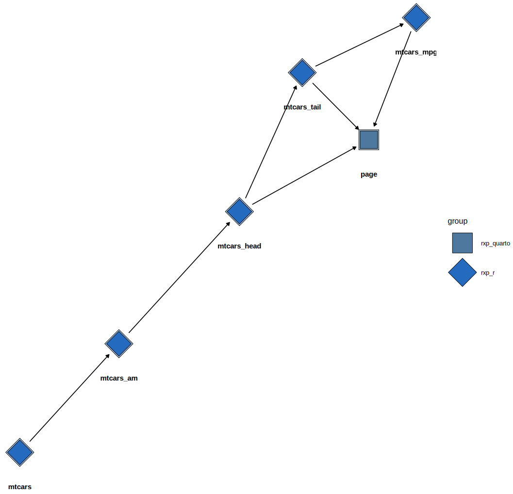
This won’t build the pipeline but will generate useful files, including a JSON representation of the pipeline at _rixpress/dag.json. This process is quick and allows you to visualize the graph using rxp_visnetwork(), which opens a new tab in your web browser displaying the pipeline’s DAG, generated using the visNetwork package:

(This image shows the DAG of a more complex example pipeline.)

For static documents, you can use rxp_ggdag() which uses ggdag under the hood:

You can also return the underlying igraph object to plot the DAG using other tools:

dag_for_ci()

which saves the dag.dot object in the project’s _rixpress/ folder.

After reviewing the DAG, you can build the pipeline by running rxp_make() instead of modifying your original rixpress() call.

Caveats

There are some caveats that you need to be aware of when using rixpress. Due to how Nix works, certain things are simply not possible:

as mentioned in vignette("a-intro-concepts"), functions are executed in a hermetic sandbox. If they need access to an external resource, the build will fail. For example, if you use a function to get data from an API, you must first retrieve the data in a standard interactive R session, save it to disk, and then include it in the pipeline. The only exception to this is rxp_r_file(), which can download a file from a URL.
all build artifacts will be saved in the Nix store, /nix/store/. If you are working with confidential data, make sure no one else can access the /nix/store.
if you have proprietary R packages, you will need to include them in the Nix shell. This is primarily a concern for rix, as it generates the execution environment. If you need help packaging your proprietary packages, please open an issue on the rix GitHub repository.

Conclusion

Now that you understand the basic, high-level concepts, let’s move on to the next vignette, vignette("c-tutorial"), where we’ll learn how to set up a pipeline from start to finish.